Typical use case for physical parameters
This example notebook shows a run on the COSMOS2020 (Weaver et al. 2022) data set in order to estimate the physical parameters.
In this notebook we follow what has been done for photo-z. We will be looking at the same COSMOS data set but only use the ugrizy bands. The main difference is the use of BC03 templates to compute physical parameters, and we set the redshift to its spectrosocpic value.
The notebook can be downloaded here.
[1]:
import lephare as lp
from astropy.table import Table
import numpy as np
import os
from matplotlib import pylab as plt
import time

%matplotlib inline
%load_ext wurlitzer
LEPHAREDIR is being set to the default cache directory:
/home/docs/.cache/lephare/data
More than 1Gb may be written there.
LEPHAREWORK is being set to the default cache directory:
/home/docs/.cache/lephare/work
Default work cache is already linked.
This is linked to the run directory:
/home/docs/.cache/lephare/runs/20260625T093605
Update the config
We will start with the COSMOS configuration as a basis. We will update the various keywords needed for this example. We use the default which is shipped with lephare. You could also download the example text file config from here or write it completely from scratch.
[2]:
config = lp.default_cosmos_config.copy()

# You could also load this from a local text file:
# config=lp.keymap_to_string_dict(lp.read_config("your_own.para"))
# An example can be downloaded with curl
# !curl -s -o ./COSMOS.para https://raw.githubusercontent.com/lephare-photoz/lephare-data/refs/heads/main/examples/COSMOS.para
# config = lp.read_config("./COSMOS.para")

config.update(
    {
        # For a quick demonstration we use a very sparse redshift grid. DO NOT USE FOR SCIENCE!
        # Comment out the following line to improve results.
        "Z_STEP": "0.1,0.,3.",
        # SED
        # In order to get the physical parameters you need to use
        # Composite Stellar Population synthesis models. Here Bruzual & Charlot (2003).
        # This can be done only for galaxies.
        "GAL_SED": "$LEPHAREDIR/sed/GAL/BC03_CHAB/BC03COMB_MOD.list",
        # Limit the number of ages
        "SEL_AGE": "$LEPHAREDIR/sed/GAL/BC03_CHAB/AGE_BC03COMB.dat",
        "MOD_EXTINC": "0,12,0,12",
        "EXTINC_LAW": "SB_calzetti.dat,SMC_prevot.dat",
        "EM_LINES": "PHYS",
        "EM_DISPERSION": "1.",
        # FILTERS
        # A reduced list of filters:
        "FILTER_LIST": "cosmos/u_new.pb,hsc/gHSC.pb,hsc/rHSC.pb,hsc/iHSC.pb,hsc/zHSC.pb,hsc/yHSC.pb",
        "FILTER_CALIB": "0",
        "FILTER_FILE": "filter_test",
        # FIT
        # We set the redshift to the spec-z value
        "ZFIX": "YES",
        "ERR_SCALE": "0.02",
        "ERR_FACTOR": "1.5",
        "SPEC_OUT": "NO",  # We would like to see the output
        "VERBOSE": "NO",
    }
)
Download the missing data
One does not need to use this functionality if already cloned the full auxiliary data.
[3]:
lp.data_retrieval.get_auxiliary_data(
    keymap=config,
    # The additional extinction laws for galaxies are not in the principle config
    # so we must add them to be downloaded:
    additional_files=[
        # We also want the example cosmos catalogue to experiment with
        "examples/COSMOS.in",
        "ext/SMC_prevot.dat",
        "ext/SB_calzetti.dat",
        "sed/GAL/BC03_CHAB/AGE_BC03COMB.dat",
    ],
)
Registry file downloaded and saved as data_registry.txt.
Downloading file 'sed/GAL/BC03_CHAB/BC03COMB_MOD.list' from 'https://raw.githubusercontent.com/lephare-photoz/lephare-data/main/sed/GAL/BC03_CHAB/BC03COMB_MOD.list' to '/home/docs/.cache/lephare/data'.
Downloading file 'sed/GAL/BC03_CHAB/bc2003_lr_m62_chab_tau01_dust00.ised_ASCII' from 'https://raw.githubusercontent.com/lephare-photoz/lephare-data/main/sed/GAL/BC03_CHAB/bc2003_lr_m62_chab_tau01_dust00.ised_ASCII' to '/home/docs/.cache/lephare/data'.
Downloading file 'sed/GAL/BC03_CHAB/bc2003_lr_m62_chab_tau3_dust00.ised_ASCII' from 'https://raw.githubusercontent.com/lephare-photoz/lephare-data/main/sed/GAL/BC03_CHAB/bc2003_lr_m62_chab_tau3_dust00.ised_ASCII' to '/home/docs/.cache/lephare/data'.
Downloading file 'sed/GAL/BC03_CHAB/bc2003_lr_m62_chab_tau03_dust00.ised_ASCII' from 'https://raw.githubusercontent.com/lephare-photoz/lephare-data/main/sed/GAL/BC03_CHAB/bc2003_lr_m62_chab_tau03_dust00.ised_ASCII' to '/home/docs/.cache/lephare/data'.
Downloading file 'sed/GAL/BC03_CHAB/bc2003_lr_m52_chab_tau5_dust00.ised_ASCII' from 'https://raw.githubusercontent.com/lephare-photoz/lephare-data/main/sed/GAL/BC03_CHAB/bc2003_lr_m52_chab_tau5_dust00.ised_ASCII' to '/home/docs/.cache/lephare/data'.
Downloading file 'sed/GAL/BC03_CHAB/bc2003_lr_m62_chab_tau1_dust00.ised_ASCII' from 'https://raw.githubusercontent.com/lephare-photoz/lephare-data/main/sed/GAL/BC03_CHAB/bc2003_lr_m62_chab_tau1_dust00.ised_ASCII' to '/home/docs/.cache/lephare/data'.
Created directory: /home/docs/.cache/lephare/data/sed/GAL/BC03_CHAB_DELAYED
Created directory: /home/docs/.cache/lephare/data/sed/GAL/BC03_CHAB
Checking/downloading 400 files...
Downloading file 'sed/GAL/BC03_CHAB/bc2003_lr_m62_chab_tau5_dust00.ised_ASCII' from 'https://raw.githubusercontent.com/lephare-photoz/lephare-data/main/sed/GAL/BC03_CHAB/bc2003_lr_m62_chab_tau5_dust00.ised_ASCII' to '/home/docs/.cache/lephare/data'.
Downloading file 'sed/GAL/BC03_CHAB/bc2003_lr_m52_chab_tau30_dust00.ised_ASCII' from 'https://raw.githubusercontent.com/lephare-photoz/lephare-data/main/sed/GAL/BC03_CHAB/bc2003_lr_m52_chab_tau30_dust00.ised_ASCII' to '/home/docs/.cache/lephare/data'.
Downloading file 'sed/GAL/BC03_CHAB/bc2003_lr_m62_chab_tau30_dust00.ised_ASCII' from 'https://raw.githubusercontent.com/lephare-photoz/lephare-data/main/sed/GAL/BC03_CHAB/bc2003_lr_m62_chab_tau30_dust00.ised_ASCII' to '/home/docs/.cache/lephare/data'.
Downloading file 'sed/GAL/BC03_CHAB_DELAYED/bc2003_lr_m52_chab_delayed1_dust00.ised_ASCII' from 'https://raw.githubusercontent.com/lephare-photoz/lephare-data/main/sed/GAL/BC03_CHAB_DELAYED/bc2003_lr_m52_chab_delayed1_dust00.ised_ASCII' to '/home/docs/.cache/lephare/data'.
Downloading file 'sed/GAL/BC03_CHAB_DELAYED/bc2003_lr_m52_chab_delayed3_dust00.ised_ASCII' from 'https://raw.githubusercontent.com/lephare-photoz/lephare-data/main/sed/GAL/BC03_CHAB_DELAYED/bc2003_lr_m52_chab_delayed3_dust00.ised_ASCII' to '/home/docs/.cache/lephare/data'.
Downloading file 'sed/GAL/BC03_CHAB_DELAYED/bc2003_lr_m62_chab_delayed1_dust00.ised_ASCII' from 'https://raw.githubusercontent.com/lephare-photoz/lephare-data/main/sed/GAL/BC03_CHAB_DELAYED/bc2003_lr_m62_chab_delayed1_dust00.ised_ASCII' to '/home/docs/.cache/lephare/data'.
Downloading file 'sed/GAL/BC03_CHAB_DELAYED/bc2003_lr_m62_chab_delayed3_dust00.ised_ASCII' from 'https://raw.githubusercontent.com/lephare-photoz/lephare-data/main/sed/GAL/BC03_CHAB_DELAYED/bc2003_lr_m62_chab_delayed3_dust00.ised_ASCII' to '/home/docs/.cache/lephare/data'.
Downloading file 'sed/GAL/BC03_CHAB/AGE_BC03COMB.dat' from 'https://raw.githubusercontent.com/lephare-photoz/lephare-data/main/sed/GAL/BC03_CHAB/AGE_BC03COMB.dat' to '/home/docs/.cache/lephare/data'.
400 completed.
All files downloaded successfully and are non-empty.
Checking/downloading 4 files...
4 completed.
All files downloaded successfully and are non-empty.
Run prepare
These are the key preparatory stages that calculate the filters in the LePHARE format, calculate the library of SEDs and finally calculate the library of magnitudes for all the models. The prepare method runs filter, sedtolib, and mag_gal that would be run independently at the command line. These are all explained in detail in the documentation.
[4]:
lp.prepare(
    config,
)
Creating the input table
We need to make an astropy table as input. This can be done using the standard column order: id, flux0, err0, flux1, err1,…, context, zspec, arbitrary_string. A simple example table with two filters might look like this: | id | flux_filt1 | fluxerr_filt1 | flux_filt2 | fluxerr_filt2 | context | zspec | string_data | |—|---|—|---|—|---|—|—| | 0 | 1.e-31 | 1.e-32 | 1.e-31 | 2.e-32 | 3 | NaN | “This is just a note” | | 1 | 2.e-31 | 1.e-32 | 1.e-31 | 2.e-32 |3 | 1. | “This has a specz” | | 2 | 2.e-31 | 1.e-32 | 2.e-31 | 2.e-32 | 2 | NaN| “This context only uses the second filter” |
The context detemermines which bands are used but can be -99 or a numpy.nan. We do not need to have units on the flux columns but LePHARE assumes they are in erg /s /cm**2 / Hz if we are using fluxes. The number of columns must be two times the number of filters plus the four additional columns.
This input table must use the standard column ordering to determine column meaning. This odering depends on the filter order in the config FILTER_LIST value.
[5]:
# Load the full cosmos example we downloaded at the start
cosmos_full = Table.read(f"{lp.LEPHAREDIR}/examples/COSMOS.in", format="ascii")
# Lets just look at the first 1000 specz between 0 and 3 to be fast and have a small sample to test
specz_colname = cosmos_full.colnames[-2]
mask = cosmos_full[specz_colname] > 0

mask &= cosmos_full[specz_colname] < 3
cosmos_full = cosmos_full[mask][:1000]
[6]:
input_table = Table()
# The id is in the first column
input_table["id"] = cosmos_full[cosmos_full.colnames[0]]
# Loop over the filters we want to keep to get the number of the filter, n, and the name, b,
filter_names = config["FILTER_LIST"].split(",")
for n, filter_name in enumerate(filter_names):
    # The ugrizy fluxes and errors are in cols 3 to 14
    f_col = cosmos_full.colnames[2 * n + 3]
    ferr_col = cosmos_full.colnames[2 * n + 4]
    # By default lephare uses column order so names are irrelevant
    input_table[f"f_{filter_name}"] = cosmos_full[f_col]
    input_table[f"ferr_{filter_name}"] = cosmos_full[ferr_col]
# The context is a binary flag. Here we set it to use all filters.
input_table["context"] = np.sum(2 ** np.arange(len(filter_names)))
input_table["zspec"] = cosmos_full[specz_colname]
input_table["string_data"] = "arbitrary_info"
[7]:
# Look at the first 5 lines of the input table
input_table[:5]
[7]:
| id | f_cosmos/u_new.pb | ferr_cosmos/u_new.pb | f_hsc/gHSC.pb | ferr_hsc/gHSC.pb | f_hsc/rHSC.pb | ferr_hsc/rHSC.pb | f_hsc/iHSC.pb | ferr_hsc/iHSC.pb | f_hsc/zHSC.pb | ferr_hsc/zHSC.pb | f_hsc/yHSC.pb | ferr_hsc/yHSC.pb | context | zspec | string_data |
|---|---|---|---|---|---|---|---|---|---|---|---|---|---|---|---|
| int64 | float64 | float64 | float64 | float64 | float64 | float64 | float64 | float64 | float64 | float64 | float64 | float64 | int64 | float64 | str14 |
| 2 | 4.232901366689564e-30 | 3.4341315142888603e-31 | 6.179738935719169e-30 | 1.386731273412228e-31 | 1.2142639224559102e-29 | 1.8245325069819158e-31 | 2.1114793014441938e-29 | 2.1601688228846318e-31 | 3.9365460376947166e-29 | 3.4133974396324463e-31 | 5.0357913173859444e-29 | 5.203234525553232e-31 | 63 | 1.166 | arbitrary_info |
| 3 | 1.8604787800453155e-28 | 3.6102558328725637e-31 | 1.0163707206619843e-27 | 2.5508479438832455e-30 | 2.5637553789165174e-27 | 3.907537695918684e-30 | 3.852181904261173e-27 | 4.270412613938428e-30 | 5.051842896248005e-27 | 5.651717781917373e-30 | 5.820737300549565e-27 | 6.786202238144557e-30 | 63 | 0.1649 | arbitrary_info |
| 6 | 3.883122772291653e-30 | 9.595010842153324e-32 | 4.647041003941889e-30 | 1.087246463423006e-31 | 4.8469179256155955e-30 | 1.178374194432367e-31 | 6.118486088007425e-30 | 1.2683990766417867e-31 | 9.150015677196151e-30 | 1.9130763838587345e-31 | 1.0166486142973662e-29 | 3.495575779500692e-31 | 63 | 1.25 | arbitrary_info |
| 9 | 2.8521064572984233e-30 | 1.897459353660885e-31 | 7.283799341197919e-30 | 1.7286878697910101e-31 | 2.3956967578910942e-29 | 2.8232988053219177e-31 | 5.597814087271151e-29 | 3.7781712042067346e-31 | 8.467793964385691e-29 | 5.472733062400153e-31 | 1.0885331971552352e-28 | 7.893832949105172e-31 | 63 | 0.6233 | arbitrary_info |
| 10 | 4.0113693940454606e-30 | 1.4061914648406559e-31 | 5.3481882134164066e-30 | 1.4193075132576959e-31 | 6.221652738450281e-30 | 1.5878330837093787e-31 | 7.330388037942477e-30 | 1.735529599561101e-31 | 1.1108868491203026e-29 | 2.6930229981999465e-31 | 1.5213763225065445e-29 | 5.031524893553477e-31 | 63 | 1.4005 | arbitrary_info |
Run process
Finally we run the main fitting process which is equivalent to zphota when using the command line. We also need to update some of the config values to make them consistent with the number of filters.
[8]:
# Compute physical parameters
output, _ = lp.process(config, input_table)
Using user columns from input table assuming they are in the standard MEME order.
Processing 1000 objects with 6 bands
AUTO_ADAPT is set to YES. Computing offsets.
# Offsets added to the modeled magnitudes (or substracted to the observed): 0.0,0.0,0.0,0.0,0.0,0.0
[9]:
# the output is an astropy tabel that can be manipulated in the standard ways.
output[:5]
[9]:
| IDENT | Z_BEST | Z_BEST68_LOW | Z_BEST68_HIGH | Z_MED | Z_MED68_LOW | Z_MED68_HIGH | CHI_BEST | MOD_BEST | EXTLAW_BEST | EBV_BEST | Z_SEC | CHI_SEC | MOD_SEC | EBV_SEC | ZQ_BEST | CHI_QSO | MOD_QSO | MOD_STAR | CHI_STAR | MAG_OBS() | ERR_MAG_OBS() | K_COR() | MAG_ABS() | EMAG_ABS() | MABS_FILT() | SCALE_BEST | NBAND_USED | CONTEXT | ZSPEC | AGE_BEST | AGE_INF | AGE_MED | AGE_SUP | LDUST_BEST | LDUST_INF | LDUST_MED | LDUST_SUP | LUM_TIR_BEST | LUM_TIR_INF | LUM_TIR_MED | LUM_TIR_SUP | MASS_BEST | MASS_INF | MASS_MED | MASS_SUP | SFR_BEST | SFR_INF | SFR_MED | SFR_SUP | SSFR_BEST | SSFR_INF | SSFR_MED | SSFR_SUP | COL1_INF | COL1_MED | COL1_SUP | COL2_INF | COL2_MED | COL2_SUP | LUM_NUV_BEST | LUM_R_BEST | LUM_K_BEST | MAG_PRED() | STRING_INPUT | PDF_BAY_ZG() |
|---|---|---|---|---|---|---|---|---|---|---|---|---|---|---|---|---|---|---|---|---|---|---|---|---|---|---|---|---|---|---|---|---|---|---|---|---|---|---|---|---|---|---|---|---|---|---|---|---|---|---|---|---|---|---|---|---|---|---|---|---|---|---|---|---|---|
| str4 | float64 | float64 | float64 | float64 | float64 | float64 | float64 | int64 | float64 | float64 | float64 | float64 | int64 | float64 | float64 | float64 | int64 | int64 | float64 | float64[6] | float64[6] | float64[6] | float64[6] | float64[6] | float64[6] | float64 | int64 | int64 | float64 | float64 | float64 | float64 | float64 | float64 | float64 | float64 | float64 | float64 | float64 | float64 | float64 | float64 | float64 | float64 | float64 | float64 | float64 | float64 | float64 | float64 | float64 | float64 | float64 | float64 | float64 | float64 | float64 | float64 | float64 | float64 | float64 | float64 | float64[0] | str14 | float64[31] |
| 2 | 1.166 | 0.0 | 3.0 | 1.2000000000000002 | 1.1319999992847445 | 1.2680000007152559 | 7.353547030322183 | 7 | 2.0 | 0.3 | -99.9 | -99.0 | -99 | -99.0 | 1.166 | 6.672257421014208 | 7 | -99 | 1000000000.0 | 24.83340462789454 .. 22.14483068826189 | 0.1355221450661712 .. 0.03439919376856379 | 1.4027514359493192 .. 0.22746431903521272 | -20.76039123476376 .. -22.595422660630916 | 0.35799910340307406 .. 3.217256181124121 | 3.0 .. 5.0 | 508394575538.1546 | 6 | 0 | 1.166 | 9.477121254719663 | 9.070826931809764 | 9.340808033918837 | 9.585138349049188 | 11.262688906793807 | 11.263775914659584 | 11.31921324390277 | 11.430530743344463 | -999.0 | -99.9 | -99.9 | -99.9 | 10.458906909307618 | 10.305498041588109 | 10.460449856228049 | 10.617354682294922 | 1.1856501725118802 | 1.1460700391298684 | 1.254851965731712 | 1.4173108543425348 | -9.273256736795737 | -9.386450745969796 | -9.182778986875206 | -8.908110590004203 | -99.9 | -99.9 | -99.9 | -99.9 | -99.9 | -99.9 | 10.098781878596972 | 10.079056546113724 | 9.26246804596414 | arbitrary_info | 0.0 .. 0.0 | |
| 3 | 0.1649 | 0.0 | 3.0 | 0.2 | 0.13199999928474426 | 0.26800000071525576 | 1.127109729785316 | 1 | 1.0 | 0.35 | -99.9 | -99.0 | -99 | -99.0 | 0.1649 | 49.54801586527253 | 1 | -99 | 1000000000.0 | 20.725938197553823 .. 16.98755500174321 | 0.03016607985901451 .. 0.030060055672664364 | 0.8065954644069318 .. 0.11396514031072706 | -19.553034052624728 .. -22.618055215012145 | 1.2252872539779265 .. 0.9043228285283575 | 1.0 .. 5.0 | 62291433485.13771 | 6 | 0 | 0.1649 | 8.85654824429995 | 8.814715058852782 | 8.882787049787268 | 9.002480837126864 | 10.946517075165014 | 11.108956976568155 | 11.162439684103527 | 11.238848432982804 | -999.0 | -99.9 | -99.9 | -99.9 | 10.597128578764885 | 10.739540782287092 | 10.781647330152634 | 10.82537362398034 | -0.3268503478547725 | -1.4055377938750317 | -0.1761292779683207 | -0.00037526675499195694 | -10.923978926619657 | -12.205537469043191 | -10.976131415901882 | -10.800382201257246 | -99.9 | -99.9 | -99.9 | -99.9 | -99.9 | -99.9 | 9.42570394618821 | 10.187058622417833 | 9.425068101607351 | arbitrary_info | 0.0 .. 0.0 | |
| 6 | 1.25 | 0.0 | 3.0 | 1.2000000000000002 | 1.1319999992847445 | 1.2680000007152559 | 0.8753132980664218 | 11 | 1.0 | 0.15 | -99.9 | -99.0 | -99 | -99.0 | 1.25 | 21.04195848639247 | 21 | -99 | 1000000000.0 | 24.92704719548275 .. 23.882072817400996 | 0.05020167671229883 .. 0.06353871767418252 | -0.16111586808040457 .. -0.21214526248971308 | -19.57709975782467 .. -20.605487428788244 | 0.3375439166770793 .. 3.6044856532246143 | 4.0 .. 5.0 | 13803624804.673458 | 6 | 0 | 1.25 | 8.85654824429995 | 8.536017876504694 | 8.803608585052846 | 9.107455083407531 | 10.581529249478102 | 10.213565216857885 | 10.489423305486685 | 10.574905411891562 | -999.0 | -99.9 | -99.9 | -99.9 | 9.19186249267866 | 8.975560033754876 | 9.115778480543227 | 9.261780580497703 | 0.684413476414361 | 0.31552402209590663 | 0.5099874640159455 | 0.6591685767866572 | -8.507449016264298 | -8.922962444876912 | -8.563317879883106 | -8.395134335338103 | -99.9 | -99.9 | -99.9 | -99.9 | -99.9 | -99.9 | 9.548654102471012 | 9.214921861147548 | 8.340639502400958 | arbitrary_info | 0.0 .. 0.0 | |
| 9 | 0.6233 | 0.0 | 3.0 | 0.6000000000000001 | 0.5319999992847443 | 0.6680000007152558 | 10.08553107425512 | 9 | 1.0 | 0.15 | -99.9 | -99.0 | -99 | -99.0 | 0.6233 | 2.1015424840408587 | 4 | -99 | 1000000000.0 | 25.262085670267126 .. 21.307895804197347 | 0.11245030713537811 .. 0.03224207737358272 | 1.3022229798649088 .. 0.3272615330764923 | -19.084924703360304 .. -21.858864579956013 | 0.26711059816815386 .. 1.7211440455862501 | 2.0 .. 5.0 | 60861552909.72918 | 6 | 0 | 0.6233 | 9.812913339271075 | 9.65004889105882 | 9.780227478802393 | 9.84483344431772 | 10.187217974697251 | 10.685450320855134 | 10.87473823552697 | 10.98375313803746 | -999.0 | -99.9 | -99.9 | -99.9 | 10.506329461182165 | 10.38953907810179 | 10.462714951008715 | 10.531521287516288 | -0.2256575514439052 | -0.48546797509497264 | -0.14889939469231891 | 0.3748550938608418 | -10.731987012626071 | -10.887791840258354 | -10.614074825331386 | -10.108976115916684 | -99.9 | -99.9 | -99.9 | -99.9 | -99.9 | -99.9 | 8.77946622163915 | 9.564947639569699 | 8.954704685600117 | arbitrary_info | 0.0 .. 0.0 | |
| 10 | 1.4005 | 0.0 | 3.0 | 1.4 | 1.3319999992847442 | 1.4680000007152556 | 0.34841120873857717 | 9 | 2.0 | 0.1 | -99.9 | -99.0 | -99 | -99.0 | 1.4005 | 35.34603210152784 | 7 | -99 | 1000000000.0 | 24.891768358503363 .. 23.444408367607465 | 0.06450552103875724 .. 0.06166419141859548 | 0.11232905902905901 .. -0.3339735279878466 | -20.218146548545384 .. -21.22658773633921 | 0.37713681002682975 .. 4.581956109462219 | 4.0 .. 5.0 | 13236946761.090946 | 6 | 0 | 1.4005 | 9.206550637652406 | 8.820118768131941 | 9.161140716627195 | 9.37385994775412 | 10.515345537095437 | 10.474474667471569 | 10.535024382445346 | 10.976592245618587 | -999.0 | -99.9 | -99.9 | -99.9 | 9.606109062415369 | 9.545139710051874 | 9.69875810142439 | 9.88057010280985 | 0.6295673335609094 | 0.5922986786488833 | 0.6958446208697591 | 0.9426267673077546 | -8.97654172885446 | -9.188513913247936 | -9.000918573678264 | -8.730313145618705 | -99.9 | -99.9 | -99.9 | -99.9 | -99.9 | -99.9 | 9.545775642862143 | 9.424650892525019 | 8.531288470037632 | arbitrary_info | 0.0 .. 0.0 |
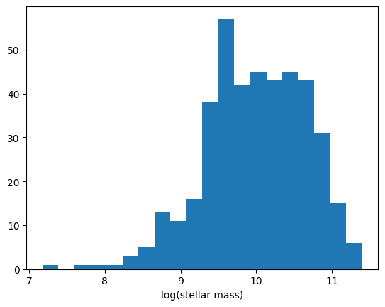
Next we can perform some simple plots to check the output
[10]:
logmass = output["MASS_MED"]
logSFR = output["SFR_MED"]
z = output["Z_BEST"]
cond = (z > 0.5) & (z < 1) & (logmass > 0)
plt.hist(logmass[cond], bins=20)
plt.xlabel("log(stellar mass)")
[10]:
Text(0.5, 0, 'log(stellar mass)')
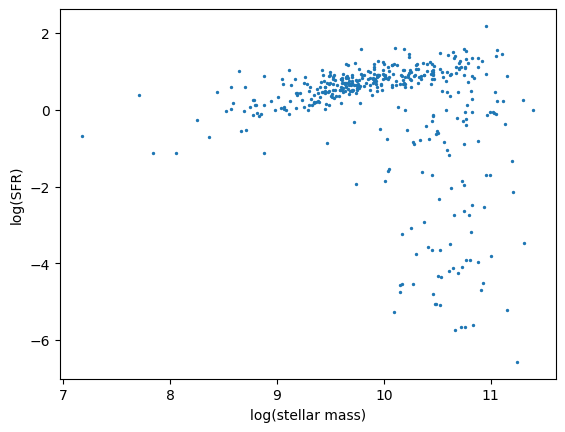
[11]:
plt.scatter(logmass[cond], logSFR[cond], s=2.0)
plt.xlabel("log(stellar mass)")
plt.ylabel("log(SFR)")
[11]:
Text(0, 0.5, 'log(SFR)')
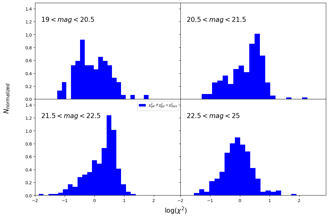
You can use some plotting utilities provided with the code. Some examples are provided below. sel_filt is the index of the filter used to select objects by observed magnitude (starting at 0). pos_filt provides the index (starting at 0) of the filters corresponding to u, g, r, z, J, and Ks bands. You can use some plotting utilities provided with the code. Some examples are provided below. If you want to create all the plots and store them in a pdf file, you can use: utils.save_phys_plots_pdf(filename=”all_phys.pdf”)
[12]:
utils = lp.PlotUtils(
    output,
    sel_filt=3,
    pos_filt=[0, 1, 2, 4, 5, 5],
    range_z=[0, 0.5, 1, 1.5, 3],
    range_mag=[19, 20.5, 21.5, 22.5, 25],
)
[13]:
utils.dist_chi2()
<Figure size 640x480 with 0 Axes>
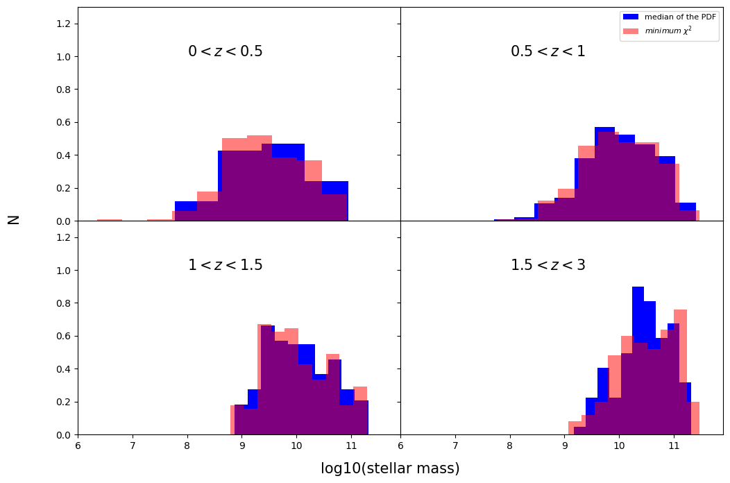
[14]:
utils.dist_mass()
<Figure size 640x480 with 0 Axes>
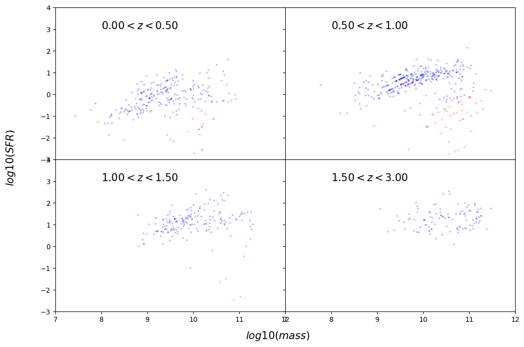
[15]:
utils.mass_sfr()
<Figure size 640x480 with 0 Axes>
[ ]: