Typical use case
In the minimal photoz run example notebook we demonstrated a run on the COSMOS2020 (Weaver et al. 2022) data set in order to show the most basic LePHARE functionality.
In this notebook we want to walk through a typical use case where the user wishes to run on a new catalogue with a new set of filters.
We will be looking at the same COSMOS data set but only use the ugrizy bands. We will take just these filters from the local auxiliary database. This should demonstrate the basic procedure for updating the configuration parameters and creating an input table in the appropriate format.
The notebook can be downloaded here.
[1]:
import lephare as lp
from astropy.table import Table
import numpy as np
import os
from matplotlib import pylab as plt
import time

%matplotlib inline
%load_ext wurlitzer
LEPHAREDIR is being set to the default cache directory:
/home/docs/.cache/lephare/data
More than 1Gb may be written there.
LEPHAREWORK is being set to the default cache directory:
/home/docs/.cache/lephare/work
Default work cache is already linked.
This is linked to the run directory:
/home/docs/.cache/lephare/runs/20260625T093605
Update the config
We will start with the COSMOS configuration as a basis. We will update the various keywords. We use the default which is shipped with lephare. You could also download the example text file config from here or write it completely from scratch.
[2]:
config = lp.default_cosmos_config.copy()

# You could also load this from a local text file:
# !curl -s -o https://raw.githubusercontent.com/lephare-photoz/lephare-data/refs/heads/main/examples/COSMOS.para
# config = lp.read_config("./COSMOS.para")

config.update(
    {
        # For a quick demonstration we use a very sparse redshift grid. DO NOT USE FOR SCIENCE!
        # Comment out the following line to improve results.
        "Z_STEP": "0.1,0.,3.",
        "VERBOSE": "NO",
    }
)
Download the required SEDs and additional extinction laws
If one has already cloned the full auxiliary data one does not need to use this functionality.
Here we will need the same set of SEDs and other files required for the COSMOS example so will download those using the automated download functionality.
[3]:
lp.data_retrieval.get_auxiliary_data(
    keymap=config,
    # The additional extinction laws for galaxies are not in the principle config
    # so we must add them to be downloaded:
    additional_files=[
        "ext/SMC_prevot.dat",
        "ext/SB_calzetti.dat",
        "ext/SB_calzetti_bump1.dat",
        "ext/SB_calzetti_bump2.dat",
        # We also want the example cosmos catalogue to experiment with
        "examples/COSMOS.in",
    ],
)
Registry file downloaded and saved as data_registry.txt.
Checking/downloading 445 files...
445 completed.
All files downloaded successfully and are non-empty.
Checking/downloading 5 files...
5 completed.
All files downloaded successfully and are non-empty.
Setting new filters
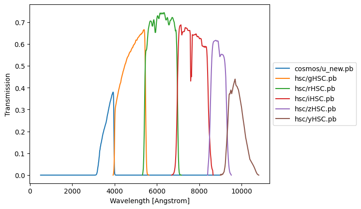
As a simple example we are taking a subset of the 30 filters used in the standard COSMOS example. To do this we will take the 6 ugrizy filters from $LEPHAREDIR/filt. To use these new filters we need to update the config and set the filter directory to their location
[4]:
# We need to update the filter list and some other config values according to the new filter list
config.update(
    {
        # A reduced list of filters:
        "FILTER_LIST": "cosmos/u_new.pb,hsc/gHSC.pb,hsc/rHSC.pb,hsc/iHSC.pb,hsc/zHSC.pb,hsc/yHSC.pb",
        # FILTER_CALIB must be updated to either have the same length as FILTER_LIST or be one number
        # ERR_SCALE and ERR_FACTOR must also be updated later to be the correct length.
        "FILTER_CALIB": "0",
        # Use a test name to avoid clashes with other runs.
        "FILTER_FILE": "filter_test",
    }
)
filter_names = config["FILTER_LIST"].split(",")
Plot the filter transmission curves.
[5]:
for n, f in enumerate(filter_names):
    data = Table.read(f"{lp.LEPHAREDIR}/filt/{f}", format="ascii")
    plt.plot(data[data.colnames[0]], data[data.colnames[1]], label=f)
plt.legend(loc="center left", bbox_to_anchor=(1, 0.5))
plt.xlabel("Wavelength [Angstrom]")
plt.ylabel("Transmission")
[5]:
Text(0, 0.5, 'Transmission')
Set specific config values for
In order to get better results we often want to use different config values for stars, galaxies and qso.
We therefore make override dictionaries for each type. These are the default configurations that were used in Ilbert et al. 2013, Laigle et al. 2016, and Weaver et al. 2022.
[6]:
# We leave stars as before
star_overrides = {}

# For galaxies we want to use a different set of extinction laws and other keyword values
gal_overrides = {
    "MOD_EXTINC": "18,26,26,33,26,33,26,33",
    "EXTINC_LAW": "SMC_prevot.dat,SB_calzetti.dat,SB_calzetti_bump1.dat,SB_calzetti_bump2.dat",
    "EM_LINES": "EMP_UV",
    "EM_DISPERSION": "0.5,1.,1.5",
}

qso_overrides = {
    "MOD_EXTINC": "0,1000",
    "EB_V": "0.,0.1,0.2,0.3",
    "EXTINC_LAW": "SB_calzetti.dat",
}
Run prepare
These are the key preparatory stages that calculate the filters in the LePHARE format, calculate the library of SEDs and finally calculate the library of magnitudes for all the models. The prepare method runs filter, sedtolib, and mag_gal that would be run independently at the command line. These are all explained in detail in the documentation.
[7]:
lp.prepare(
    config,
    star_config=star_overrides,
    gal_config=gal_overrides,
    qso_config=qso_overrides,
)
Creating the input table
We need to make an astropy table as input. This can be done using the standard column order: id, flux0, err0, flux1, err1,…, context, zspec, arbitrary_string. A simple example table with two filters might look like this: | id | flux_filt1 | fluxerr_filt1 | flux_filt2 | fluxerr_filt2 | context | zspec | string_data | |—|---|—|---|—|---|—|—| | 0 | 1.e-31 | 1.e-32 | 1.e-31 | 2.e-32 | 3 | NaN | “This is just a note” | | 1 | 2.e-31 | 1.e-32 | 1.e-31 | 2.e-32 |3 | 1. | “This has a specz” | | 2 | 2.e-31 | 1.e-32 | 2.e-31 | 2.e-32 | 2 | NaN| “This context only uses the second filter” |
The context detemermines which bands are used but can be -99 or a numpy.nan. We do not need to have units on the flux columns but LePHARE assumes they are in erg /s /cm**2 / Hz if we are using fluxes. The number of columns must be two times the number of filters plus the four additional columns.
This input table must use the standard column ordering to determine column meaning. This odering depends on the filter order in the config FILTER_LIST value.
[8]:
# Load the full cosmos example we downloaded at the start
cosmos_full = Table.read(f"{lp.LEPHAREDIR}/examples/COSMOS.in", format="ascii")
# Lets just look at the first 1000 specz between 0 and 3 to be fast and have a small sample to test
specz_colname = cosmos_full.colnames[-2]
mask = cosmos_full[specz_colname] > 0
mask &= cosmos_full[specz_colname] < 3
cosmos_full = cosmos_full[mask][:1000]
[9]:
input_table = Table()
# The id is in the first column
input_table["id"] = cosmos_full[cosmos_full.colnames[0]]
# Loop over the filters we want to keep to get the number of the filter, n, and the name, b,
for n, filter_name in enumerate(filter_names):
    # The ugrizy fluxes and errors are in cols 3 to 14
    f_col = cosmos_full.colnames[2 * n + 3]
    ferr_col = cosmos_full.colnames[2 * n + 4]
    # By default lephare uses column order so names are irrelevant
    input_table[f"f_{filter_name}"] = cosmos_full[f_col]
    input_table[f"ferr_{filter_name}"] = cosmos_full[ferr_col]
# The context is a binary flag. Here we set it to use all filters.
input_table["context"] = np.sum(2 ** np.arange(len(filter_names)))
input_table["zspec"] = cosmos_full[specz_colname]
input_table["string_data"] = "arbitrary_info"
[10]:
# Look at the first 5 lines of the input table
input_table[:5]
[10]:
| id | f_cosmos/u_new.pb | ferr_cosmos/u_new.pb | f_hsc/gHSC.pb | ferr_hsc/gHSC.pb | f_hsc/rHSC.pb | ferr_hsc/rHSC.pb | f_hsc/iHSC.pb | ferr_hsc/iHSC.pb | f_hsc/zHSC.pb | ferr_hsc/zHSC.pb | f_hsc/yHSC.pb | ferr_hsc/yHSC.pb | context | zspec | string_data |
|---|---|---|---|---|---|---|---|---|---|---|---|---|---|---|---|
| int64 | float64 | float64 | float64 | float64 | float64 | float64 | float64 | float64 | float64 | float64 | float64 | float64 | int64 | float64 | str14 |
| 2 | 4.232901366689564e-30 | 3.4341315142888603e-31 | 6.179738935719169e-30 | 1.386731273412228e-31 | 1.2142639224559102e-29 | 1.8245325069819158e-31 | 2.1114793014441938e-29 | 2.1601688228846318e-31 | 3.9365460376947166e-29 | 3.4133974396324463e-31 | 5.0357913173859444e-29 | 5.203234525553232e-31 | 63 | 1.166 | arbitrary_info |
| 3 | 1.8604787800453155e-28 | 3.6102558328725637e-31 | 1.0163707206619843e-27 | 2.5508479438832455e-30 | 2.5637553789165174e-27 | 3.907537695918684e-30 | 3.852181904261173e-27 | 4.270412613938428e-30 | 5.051842896248005e-27 | 5.651717781917373e-30 | 5.820737300549565e-27 | 6.786202238144557e-30 | 63 | 0.1649 | arbitrary_info |
| 6 | 3.883122772291653e-30 | 9.595010842153324e-32 | 4.647041003941889e-30 | 1.087246463423006e-31 | 4.8469179256155955e-30 | 1.178374194432367e-31 | 6.118486088007425e-30 | 1.2683990766417867e-31 | 9.150015677196151e-30 | 1.9130763838587345e-31 | 1.0166486142973662e-29 | 3.495575779500692e-31 | 63 | 1.25 | arbitrary_info |
| 9 | 2.8521064572984233e-30 | 1.897459353660885e-31 | 7.283799341197919e-30 | 1.7286878697910101e-31 | 2.3956967578910942e-29 | 2.8232988053219177e-31 | 5.597814087271151e-29 | 3.7781712042067346e-31 | 8.467793964385691e-29 | 5.472733062400153e-31 | 1.0885331971552352e-28 | 7.893832949105172e-31 | 63 | 0.6233 | arbitrary_info |
| 10 | 4.0113693940454606e-30 | 1.4061914648406559e-31 | 5.3481882134164066e-30 | 1.4193075132576959e-31 | 6.221652738450281e-30 | 1.5878330837093787e-31 | 7.330388037942477e-30 | 1.735529599561101e-31 | 1.1108868491203026e-29 | 2.6930229981999465e-31 | 1.5213763225065445e-29 | 5.031524893553477e-31 | 63 | 1.4005 | arbitrary_info |
Run process
Finally we run the main fitting process which is equivalent to zphota when using the command line. We also need to update some of the config values to make them consistent with the number of filters.
[11]:
# We will update some of the config parameters that are used during the fitting process
config.update(
    {
        # We turn on Auto adapt which uses spectroscopic redshifts to calculate zero-point
        # offsets which is crucial to getting good results.
        "AUTO_ADAPT": "YES",
        # The following measurements will correspond to all filters.
        # We could have an array of values for each.
        # If we have an array care must be taken to ensure it has a consistent length.
        "ERR_SCALE": "0.02",
        "ERR_FACTOR": "1.5",
        "SPEC_OUT": "save_spec",  # We would like to see the output
    }
)
[12]:
# Calculate the photometric redshifts
output, _ = lp.process(config, input_table)
Using user columns from input table assuming they are in the standard MEME order.
Processing 1000 objects with 6 bands
AUTO_ADAPT is set to YES. Computing offsets.
# Offsets added to the modeled magnitudes (or substracted to the observed): -0.006415948315602549,-0.022514709124404675,-0.024575978486680583,-0.013354288336966391,-0.016412915733994282,-0.011527028462730016
[13]:
# the output is an astropy tabel that can be manipulated in the standard ways.
output[:5]
[13]:
| IDENT | Z_BEST | Z_BEST68_LOW | Z_BEST68_HIGH | Z_MED | Z_MED68_LOW | Z_MED68_HIGH | CHI_BEST | MOD_BEST | EXTLAW_BEST | EBV_BEST | Z_SEC | CHI_SEC | MOD_SEC | EBV_SEC | ZQ_BEST | CHI_QSO | MOD_QSO | MOD_STAR | CHI_STAR | MAG_OBS() | ERR_MAG_OBS() | K_COR() | MAG_ABS() | EMAG_ABS() | MABS_FILT() | SCALE_BEST | NBAND_USED | CONTEXT | ZSPEC | AGE_BEST | AGE_INF | AGE_MED | AGE_SUP | LDUST_BEST | LDUST_INF | LDUST_MED | LDUST_SUP | LUM_TIR_BEST | LUM_TIR_INF | LUM_TIR_MED | LUM_TIR_SUP | MASS_BEST | MASS_INF | MASS_MED | MASS_SUP | SFR_BEST | SFR_INF | SFR_MED | SFR_SUP | SSFR_BEST | SSFR_INF | SSFR_MED | SSFR_SUP | COL1_INF | COL1_MED | COL1_SUP | COL2_INF | COL2_MED | COL2_SUP | LUM_NUV_BEST | LUM_R_BEST | LUM_K_BEST | MAG_PRED() | STRING_INPUT | PDF_BAY_ZG() |
|---|---|---|---|---|---|---|---|---|---|---|---|---|---|---|---|---|---|---|---|---|---|---|---|---|---|---|---|---|---|---|---|---|---|---|---|---|---|---|---|---|---|---|---|---|---|---|---|---|---|---|---|---|---|---|---|---|---|---|---|---|---|---|---|---|---|
| str4 | float64 | float64 | float64 | float64 | float64 | float64 | float64 | int64 | float64 | float64 | float64 | float64 | int64 | float64 | float64 | float64 | int64 | int64 | float64 | float64[6] | float64[6] | float64[6] | float64[6] | float64[6] | float64[6] | float64 | int64 | int64 | float64 | float64 | float64 | float64 | float64 | float64 | float64 | float64 | float64 | float64 | float64 | float64 | float64 | float64 | float64 | float64 | float64 | float64 | float64 | float64 | float64 | float64 | float64 | float64 | float64 | float64 | float64 | float64 | float64 | float64 | float64 | float64 | float64 | float64 | float64[0] | str14 | float64[31] |
| 2 | 1.1218955184149433 | 1.0889679594803516 | 1.128221629704656 | 1.1196836338809963 | 1.0386401743141833 | 1.1907245950224365 | 5.3070056103377805 | 24 | 1.0 | 0.25 | -99.9 | -99.0 | -99 | -99.0 | 1.0922123964794657 | 2.9481492433922716 | 20 | 137 | 148.80879509861504 | 24.83982057621014 .. 22.15635771672462 | 0.1355221450661712 .. 0.03439919376856379 | 1.1417163010377056 .. 0.02192004320962047 | -20.56171925910113 .. -22.274737695954215 | 0.246018702985495 .. 2.492788034574822 | 3.0 .. 5.0 | 818.6911496061373 | 6 | 0 | 1.166 | -999.0 | -99.9 | -99.9 | -99.9 | -999.0 | -99.9 | -99.9 | -99.9 | -999.0 | -99.9 | -99.9 | -99.9 | -999.0 | -99.9 | -99.9 | -99.9 | -999.0 | -99.9 | -99.9 | -99.9 | -999.0 | -99.9 | -99.9 | -99.9 | -99.9 | -99.9 | -99.9 | -99.9 | -99.9 | -99.9 | 9.876707562694527 | 9.931411249844032 | 9.108603305302658 | arbitrary_info | 1.5827063703841973e-29 .. 2.4448941451569878e-132 | |
| 3 | 0.1487273033996954 | 0.09939903675737691 | 0.14661871523214118 | 0.136708522790407 | 0.05042594607183258 | 0.21367803680689393 | 26.4900675246165 | 20 | 1.0 | 0.5 | -99.9 | -99.0 | -99 | -99.0 | 0.07562069968044695 | 18.796540407765942 | 9 | 106 | 131.91891956063543 | 20.732354145869422 .. 16.99908203020594 | 0.03016607985901451 .. 0.030060055672664364 | 0.5427106318716775 .. 0.19231573697642873 | -19.256798236490397 .. -22.43897421671174 | 0.7389966465201248 .. 0.5285395532939319 | 1.0 .. 5.0 | 664.0969614604708 | 6 | 0 | 0.1649 | -999.0 | -99.9 | -99.9 | -99.9 | -999.0 | -99.9 | -99.9 | -99.9 | -999.0 | -99.9 | -99.9 | -99.9 | -999.0 | -99.9 | -99.9 | -99.9 | -999.0 | -99.9 | -99.9 | -99.9 | -999.0 | -99.9 | -99.9 | -99.9 | -99.9 | -99.9 | -99.9 | -99.9 | -99.9 | -99.9 | 9.613281869905844 | 10.008737854670791 | 9.393074928373007 | arbitrary_info | 2.516880514905794e-36 .. 0.0 | |
| 6 | 1.1878684779170439 | 1.1568892343966624 | 1.2262755364830291 | 1.239314453777919 | 1.1328838652015214 | 1.7381338213135793 | 1.1050012761768413 | 29 | 2.0 | 0.2 | -99.9 | -99.0 | -99 | -99.0 | 1.7431004953762879 | 7.472441641155649 | 4 | 239 | 217.88340102971432 | 24.93346314379835 .. 23.893599845863726 | 0.05020167671229883 .. 0.06353871767418252 | -0.21831145915553687 .. -0.3655571916682442 | -19.42735047385369 .. -20.303562917620326 | 0.246018702985495 .. 2.492788034574822 | 3.0 .. 5.0 | 282.65016006570863 | 6 | 0 | 1.25 | -999.0 | -99.9 | -99.9 | -99.9 | -999.0 | -99.9 | -99.9 | -99.9 | -999.0 | -99.9 | -99.9 | -99.9 | -999.0 | -99.9 | -99.9 | -99.9 | -999.0 | -99.9 | -99.9 | -99.9 | -999.0 | -99.9 | -99.9 | -99.9 | -99.9 | -99.9 | -99.9 | -99.9 | -99.9 | -99.9 | 9.649381737085797 | 9.261673826300871 | 8.22726198142654 | arbitrary_info | 1.1688399597214769e-19 .. 6.623604588076765e-82 | |
| 9 | 0.6017875067598892 | 0.5893126130383511 | 0.6114798693725609 | 0.6004069487148301 | 0.5319378082053182 | 0.6685991328409743 | 8.734630795757614 | 18 | 1.0 | 0.35 | -99.9 | -99.0 | -99 | -99.0 | 0.5770143521481803 | 3.076554463355609 | 5 | 118 | 55.272715449568786 | 25.268501618582725 .. 21.319422832660077 | 0.11245030713537811 .. 0.03224207737358272 | 1.5318768385731205 .. 0.4954761655349847 | -18.89049932975761 .. -21.92288498831445 | 0.15821443857047335 .. 1.4060958792660188 | 2.0 .. 5.0 | 295.41232875934395 | 6 | 0 | 0.6233 | -999.0 | -99.9 | -99.9 | -99.9 | -999.0 | -99.9 | -99.9 | -99.9 | -999.0 | -99.9 | -99.9 | -99.9 | -999.0 | -99.9 | -99.9 | -99.9 | -999.0 | -99.9 | -99.9 | -99.9 | -999.0 | -99.9 | -99.9 | -99.9 | -99.9 | -99.9 | -99.9 | -99.9 | -99.9 | -99.9 | 9.19927575445378 | 9.65659403966946 | 9.133851139239695 | arbitrary_info | 1.6283294325909342e-135 .. 0.0 | |
| 10 | 1.4021590748429256 | 1.384126028641362 | 1.417306765231467 | 1.4336668656412341 | 1.3409476141324919 | 1.9161188151443402 | 0.40546919172745427 | 26 | 1.0 | 0.1 | -99.9 | -99.0 | -99 | -99.0 | 1.8091440983215408 | 8.351948273108537 | 1 | 53 | 178.51081607671676 | 24.898184306818962 .. 23.455935396070196 | 0.06450552103875724 .. 0.06166419141859548 | 0.06467088707576632 .. -0.4855025961866429 | -20.226787851633457 .. -21.066708446111903 | 0.22627949036029626 .. 3.382734204440993 | 4.0 .. 5.0 | 310.92145243379235 | 6 | 0 | 1.4005 | -999.0 | -99.9 | -99.9 | -99.9 | -999.0 | -99.9 | -99.9 | -99.9 | -999.0 | -99.9 | -99.9 | -99.9 | -999.0 | -99.9 | -99.9 | -99.9 | -999.0 | -99.9 | -99.9 | -99.9 | -999.0 | -99.9 | -99.9 | -99.9 | -99.9 | -99.9 | -99.9 | -99.9 | -99.9 | -99.9 | 9.539064008989978 | 9.426854907975951 | 8.46910403942665 | arbitrary_info | 1.5226959689656272e-15 .. 1.451098944362241e-56 |
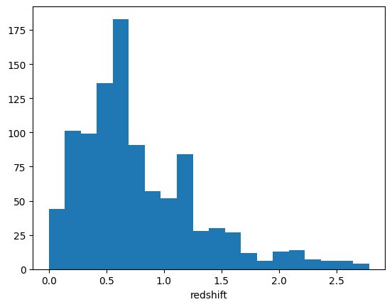
Next we can perform some simple plots to check the output
[14]:
plt.hist(output["Z_BEST"], bins=20)
plt.xlabel("redshift")
[14]:
Text(0.5, 0, 'redshift')
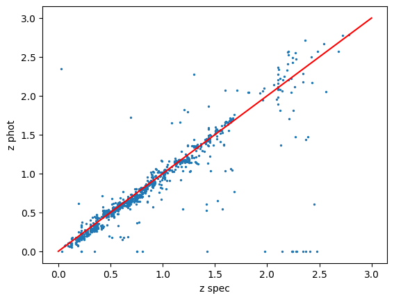
[15]:
plt.plot([0, 3], [0, 3], c="r")
plt.scatter(output["ZSPEC"], output["Z_BEST"], s=2.0)
plt.xlabel("z spec")
plt.ylabel("z phot")
[15]:
Text(0, 0.5, 'z phot')
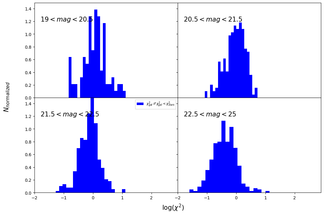
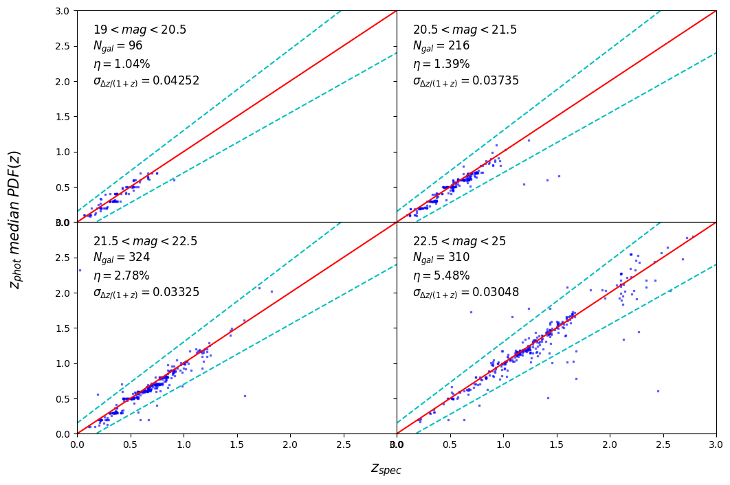
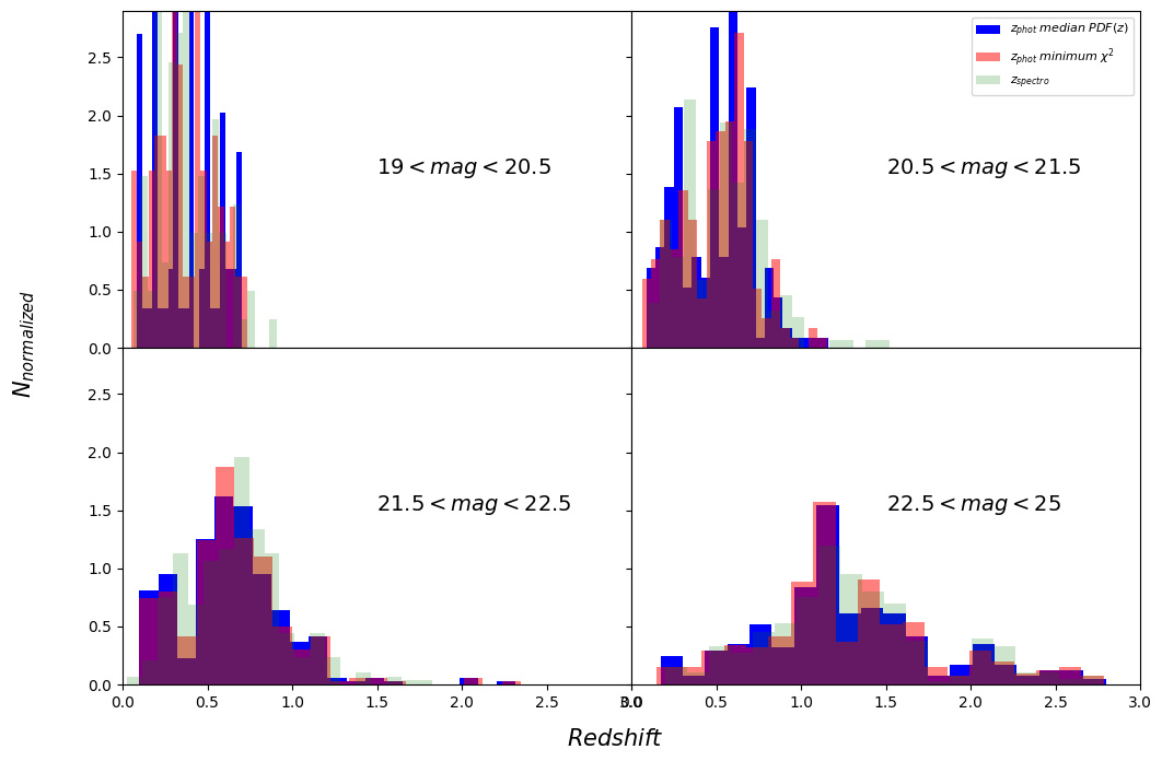
You can use some plotting utilities provided with the code. Some examples are provided below. sel_filt is the index of the filter used to select objects by observed magnitude (starting at 0). pos_filt provides the index (starting at 0) of the filters corresponding to u, g, r, z, J, and Ks bands. If you want to create all the plots and store them in a pdf file, you can use: utils.save_photoz_plots_pdf(filename=”all_photoz.pdf”)
[16]:
utils = lp.PlotUtils(
    output,
    sel_filt=3,
    pos_filt=[0, 1, 2, 4, -1, -1],
    range_z=[0, 0.5, 1, 1.5, 3],
    range_mag=[19, 20.5, 21.5, 22.5, 25],
)
Warning: pos_filt[4] out of bounds. Setting to 0.
Warning: pos_filt[5] out of bounds. Setting to 0.
[17]:
utils.dist_chi2()
<Figure size 640x480 with 0 Axes>
[18]:
utils.zml_zs()
<Figure size 640x480 with 0 Axes>
[19]:
utils.dist_z()
<Figure size 640x480 with 0 Axes>
[ ]: