Detailed run
An example of a complete run of lephare with all stages required to estimate redshift. In contrast to the two first notebooks we are not using the high level prepare and process methods. Instead we are using the more fundamental filter, sedtolib, mag_gal, and zphota which more resembles a command line based run.
We show how to include new filters from the Spanish Virtual Observatory (SVO).
Again this notebook uses the COSMOS2020 (Weaver et al. 2022) data as an example.
The notebook can be downloaded here.
[1]:
import os
import lephare as lp
import numpy as np
from matplotlib import pylab as plt

%matplotlib inline
LEPHAREDIR is being set to the default cache directory:
/home/docs/.cache/lephare/data
More than 1Gb may be written there.
LEPHAREWORK is being set to the default cache directory:
/home/docs/.cache/lephare/work
Default work cache is already linked.
This is linked to the run directory:
/home/docs/.cache/lephare/runs/20260701T060402
Set up the parameters
As for the previous notebooks we are starting with the default COSMOS config that ships with the lephare Python code.
Modification of three keywords of the parameter file.
[2]:
# Default config from COSMOS
config = lp.default_cosmos_config.copy()

# You could also load this from a local text file:
# config=lp.keymap_to_string_dict(lp.read_config("your_own.para"))
# An example can be downloaded with curl
# !curl -s -o ./COSMOS.para https://raw.githubusercontent.com/lephare-photoz/lephare-data/refs/heads/main/examples/COSMOS.para
# config = lp.read_config("./COSMOS.para")

# update keywords
config.update(
    {
        # Verbose must be NO in the notebook.
        "VERBOSE": "NO",
        # this line reduced the zgrid density from the default to make the notebook run faster.
        # Comment this out for better science results
        "Z_STEP": "0.04,0.,6.",
    }
)
Then we get the auxiliary files required to run the notebook for the documentation. If you have cloned the full auxiliary data repository you do not need to run this.
[3]:
lp.data_retrieval.get_auxiliary_data(
    keymap=config,
    additional_files=["examples/COSMOS.in", "examples/config_svo_filters.yml", "examples/output.para"],
)
Local registry file is up to date: data_registry.txt
Checking/downloading 445 files...
445 completed.
All files downloaded successfully and are non-empty.
Downloading file 'examples/config_svo_filters.yml' from 'https://raw.githubusercontent.com/lephare-photoz/lephare-data/main/examples/config_svo_filters.yml' to '/home/docs/.cache/lephare/data'.
Checking/downloading 3 files...
3 completed.
All files downloaded successfully and are non-empty.
Create filter library
Read the filter names to be used in COSMOS.para and generate the filter file
First, you can use the standard method with the list of filters in the parameter file. The filters are store in the LEPHAREDIR/filt directory. You can pass either the config file or the keymap as argument
Getting new filters
Each filter requires a filter response curve. This is a table of wavelength values in Angstrom and filter transmission in arbitrary units. In this example we get the filters we need from the SVO. We could have also used the filters that are available in $LEPHAREDIR/filt. Or one could also use local files.
[4]:
# This would get the filters from the config file and local LEPHAREDIR/filt location.
# Later we see how to do the same from the SVO.
filterRunner = lp.Filter(config_keymap=lp.all_types_to_keymap(config))
filterLib = filterRunner.run()
# NAME                        IDENT      Lbda_mean Lbeff(Vega)       FWHM     AB-cor    TG-cor      VEGA M_sun(AB)   CALIB      Lb_eff    Fac_corr
u_cfht.lowres                 1             0.3844      0.3908      0.0538    0.3150   -0.3891  -20.6345    6.0327       0      0.3815      1.0000
u_new.pb                      2             0.3690      0.3750      0.0456    0.6195   -0.2745  -20.8527    6.3135       0      0.3668      1.0000
gHSC.pb                       3             0.4851      0.4760      0.1194   -0.0860   -0.2458  -20.7272    5.0764       0      0.4780      1.0000
rHSC.pb                       4             0.6241      0.6142      0.1539    0.1466    0.2580  -21.5143    4.6523       0      0.6178      1.0000
iHSC.pb                       5             0.7716      0.7637      0.1476    0.3942    0.6138  -22.2286    4.5323       0      0.7666      1.0000
zHSC.pb                       6             0.8915      0.8907      0.0768    0.5169    0.7625  -22.6733    4.5147       0      0.8903      1.0000
yHSC.pb                       7             0.9801      0.9771      0.0797    0.5534    0.7763  -22.9145    4.5081       0      0.9782      1.0000
Y.lowres                      8             1.0222      1.0196      0.0919    0.6043    0.8180  -23.0574    4.5130       0      1.0206      1.0000
J.lowres                      9             1.2555      1.2481      0.1712    0.9228  -99.0000  -23.8194    4.5638       0      1.2514      1.0000
H.lowres                      10            1.6497      1.6352      0.2893    1.3701  -99.0000  -24.8565    4.7045       0      1.6409      1.0000
K.lowres                      11            2.1577      2.1435      0.2926    1.8335  -99.0000  -25.9057    5.1316       0      2.1502      1.0000
IB427.lowres                  12            0.4264      0.4256      0.0207   -0.1446   -0.4942  -20.4117    5.5152       0      0.4262      1.0000
IB464.lowres                  13            0.4636      0.4633      0.0218   -0.1520   -0.3463  -20.5860    5.0658       0      0.4634      1.0000
IB484.lowres                  14            0.4851      0.4846      0.0228   -0.0241   -0.1770  -20.8122    4.9880       0      0.4849      1.0000
IB505.lowres                  15            0.5064      0.5061      0.0231   -0.0656   -0.1366  -20.8639    4.9423       0      0.5061      1.0000
IB527.lowres                  16            0.5262      0.5259      0.0242   -0.0260   -0.0464  -20.9871    4.8937       0      0.5260      1.0000
IB574.lowres                  17            0.5766      0.5762      0.0272    0.0657    0.1377  -21.2773    4.7042       0      0.5763      1.0000
IB624.lowres                  18            0.6234      0.6230      0.0301    0.1527    0.2768  -21.5339    4.6386       0      0.6232      1.0000
IB679.lowres                  19            0.6783      0.6779      0.0336    0.2542    0.4288  -21.8183    4.5709       0      0.6779      1.0000
IB709.lowres                  20            0.7075      0.7071      0.0316    0.2982    0.4968  -21.9541    4.5558       0      0.7072      1.0000
IB738.lowres                  21            0.7363      0.7358      0.0323    0.3460    0.5577  -22.0886    4.5449       0      0.7360      1.0000
IB767.lowres                  22            0.7687      0.7681      0.0364    0.3992    0.6164  -22.2351    4.5243       0      0.7683      1.0000
IB827.lowres                  23            0.8246      0.8241      0.0344    0.4891    0.7300  -22.4777    4.5161       0      0.8243      1.0000
NB711.lowres                  24            0.7120      0.7119      0.0073    0.3072    0.5084  -21.9774    4.5542       0      0.7120      1.0000
NB816.lowres                  25            0.8150      0.8149      0.0120    0.4713    0.7098  -22.4349    4.5154       0      0.8149      1.0000
NB118.lowres                  26            1.1909      1.1909      0.0112    0.8376  -99.0000  -23.6250    4.5554       0      1.1909      1.0000
irac_ch1.lowres               27            3.5763      3.5264      0.7411    2.7951  -99.0000  -27.9585    6.0679       1      3.5634      1.0036
irac_ch2.lowres               28            4.5290      4.4609      1.0105    3.2634  -99.0000  -28.9384    6.5680       1      4.5111      1.0040
irac_ch3.lowres               29            5.7873      5.6765      1.3509    3.7537  -99.0000  -29.9581    7.0472       1      5.7592      1.0050
irac_ch4.lowres               30            8.0442      7.7033      2.8394    4.3959  -99.0000  -31.2962    7.6701       1      7.9590      1.0110
It is also possible to pass all the necessary keywords as arguments to the constructor:
[5]:
# the config keymap from a config file can also be added to the constructor's arguments, in which case the keywords
# will be overridden by the explicit keywords passed as arguments below.
filterRunner2 = lp.Filter(
    FILTER_REP=os.path.join(os.environ["LEPHAREDIR"], "filt"),
    FILTER_LIST="cosmos/u_cfht.lowres,cosmos/u_new.pb,hsc/gHSC.pb,hsc/rHSC.pb,\
                       hsc/iHSC.pb,hsc/zHSC.pb,hsc/yHSC.pb,vista/Y.lowres,vista/J.lowres,vista/H.lowres,\
                       vista/K.lowres,cosmos/IB427.lowres,cosmos/IB464.lowres,cosmos/IB484.lowres,\
                       cosmos/IB505.lowres,cosmos/IB527.lowres,cosmos/IB574.lowres,cosmos/IB624.lowres,\
                       cosmos/IB679.lowres,cosmos/IB709.lowres,cosmos/IB738.lowres,cosmos/IB767.lowres,\
                       cosmos/IB827.lowres,cosmos/NB711.lowres,cosmos/NB816.lowres,vista/NB118.lowres,\
                       cosmos/irac_ch1.lowres,cosmos/irac_ch2.lowres,cosmos/irac_ch3.lowres,cosmos/irac_ch4.lowres",
    TRANS_TYPE=1,
    FILTER_CALIB="0,0,0,0,0,0,0,0,0,0,0,0,0,0,0,0,0,0,0,0,0,0,0,0,0,0,1,1,1,1",
    FILTER_FILE="filter_cosmos",
)
filterLib2 = filterRunner2.run()
# NAME                        IDENT      Lbda_mean Lbeff(Vega)       FWHM     AB-cor    TG-cor      VEGA M_sun(AB)   CALIB      Lb_eff    Fac_corr
u_cfht.lowres                 1             0.3844      0.3908      0.0538    0.3150   -0.3891  -20.6345    6.0327       0      0.3815      1.0000
u_new.pb                      2             0.3690      0.3750      0.0456    0.6195   -0.2745  -20.8527    6.3135       0      0.3668      1.0000
gHSC.pb                       3             0.4851      0.4760      0.1194   -0.0860   -0.2458  -20.7272    5.0764       0      0.4780      1.0000
rHSC.pb                       4             0.6241      0.6142      0.1539    0.1466    0.2580  -21.5143    4.6523       0      0.6178      1.0000
iHSC.pb                       5             0.7716      0.7637      0.1476    0.3942    0.6138  -22.2286    4.5323       0      0.7666      1.0000
zHSC.pb                       6             0.8915      0.8907      0.0768    0.5169    0.7625  -22.6733    4.5147       0      0.8903      1.0000
yHSC.pb                       7             0.9801      0.9771      0.0797    0.5534    0.7763  -22.9145    4.5081       0      0.9782      1.0000
Y.lowres                      8             1.0222      1.0196      0.0919    0.6043    0.8180  -23.0574    4.5130       0      1.0206      1.0000
J.lowres                      9             1.2555      1.2481      0.1712    0.9228  -99.0000  -23.8194    4.5638       0      1.2514      1.0000
H.lowres                      10            1.6497      1.6352      0.2893    1.3701  -99.0000  -24.8565    4.7045       0      1.6409      1.0000
K.lowres                      11            2.1577      2.1435      0.2926    1.8335  -99.0000  -25.9057    5.1316       0      2.1502      1.0000
IB427.lowres                  12            0.4264      0.4256      0.0207   -0.1446   -0.4942  -20.4117    5.5152       0      0.4262      1.0000
IB464.lowres                  13            0.4636      0.4633      0.0218   -0.1520   -0.3463  -20.5860    5.0658       0      0.4634      1.0000
IB484.lowres                  14            0.4851      0.4846      0.0228   -0.0241   -0.1770  -20.8122    4.9880       0      0.4849      1.0000
IB505.lowres                  15            0.5064      0.5061      0.0231   -0.0656   -0.1366  -20.8639    4.9423       0      0.5061      1.0000
IB527.lowres                  16            0.5262      0.5259      0.0242   -0.0260   -0.0464  -20.9871    4.8937       0      0.5260      1.0000
IB574.lowres                  17            0.5766      0.5762      0.0272    0.0657    0.1377  -21.2773    4.7042       0      0.5763      1.0000
IB624.lowres                  18            0.6234      0.6230      0.0301    0.1527    0.2768  -21.5339    4.6386       0      0.6232      1.0000
IB679.lowres                  19            0.6783      0.6779      0.0336    0.2542    0.4288  -21.8183    4.5709       0      0.6779      1.0000
IB709.lowres                  20            0.7075      0.7071      0.0316    0.2982    0.4968  -21.9541    4.5558       0      0.7072      1.0000
IB738.lowres                  21            0.7363      0.7358      0.0323    0.3460    0.5577  -22.0886    4.5449       0      0.7360      1.0000
IB767.lowres                  22            0.7687      0.7681      0.0364    0.3992    0.6164  -22.2351    4.5243       0      0.7683      1.0000
IB827.lowres                  23            0.8246      0.8241      0.0344    0.4891    0.7300  -22.4777    4.5161       0      0.8243      1.0000
NB711.lowres                  24            0.7120      0.7119      0.0073    0.3072    0.5084  -21.9774    4.5542       0      0.7120      1.0000
NB816.lowres                  25            0.8150      0.8149      0.0120    0.4713    0.7098  -22.4349    4.5154       0      0.8149      1.0000
NB118.lowres                  26            1.1909      1.1909      0.0112    0.8376  -99.0000  -23.6250    4.5554       0      1.1909      1.0000
irac_ch1.lowres               27            3.5763      3.5264      0.7411    2.7951  -99.0000  -27.9585    6.0679       1      3.5634      1.0036
irac_ch2.lowres               28            4.5290      4.4609      1.0105    3.2634  -99.0000  -28.9384    6.5680       1      4.5111      1.0040
irac_ch3.lowres               29            5.7873      5.6765      1.3509    3.7537  -99.0000  -29.9581    7.0472       1      5.7592      1.0050
irac_ch4.lowres               30            8.0442      7.7033      2.8394    4.3959  -99.0000  -31.2962    7.6701       1      7.9590      1.0110
Second, you can use the filterSvc helper class to gain more freedom. This class allows to retrieve the list of filt objetcs, independently of writing them on file.
[6]:
filterLib = lp.FilterSvc.from_keymap(lp.all_types_to_keymap(config))
filter_output = os.path.join(os.environ["LEPHAREWORK"], "filt", config["FILTER_FILE"])
lp.write_output_filter(filter_output + ".dat", filter_output + ".doc", filterLib)
# NAME                        IDENT      Lbda_mean Lbeff(Vega)       FWHM     AB-cor    TG-cor      VEGA M_sun(AB)   CALIB      Lb_eff    Fac_corr
u_cfht.lowres                 1             0.3844      0.3908      0.0538    0.3150   -0.3891  -20.6345    6.0327       0      0.3815      1.0000
u_new.pb                      2             0.3690      0.3750      0.0456    0.6195   -0.2745  -20.8527    6.3135       0      0.3668      1.0000
gHSC.pb                       3             0.4851      0.4760      0.1194   -0.0860   -0.2458  -20.7272    5.0764       0      0.4780      1.0000
rHSC.pb                       4             0.6241      0.6142      0.1539    0.1466    0.2580  -21.5143    4.6523       0      0.6178      1.0000
iHSC.pb                       5             0.7716      0.7637      0.1476    0.3942    0.6138  -22.2286    4.5323       0      0.7666      1.0000
zHSC.pb                       6             0.8915      0.8907      0.0768    0.5169    0.7625  -22.6733    4.5147       0      0.8903      1.0000
yHSC.pb                       7             0.9801      0.9771      0.0797    0.5534    0.7763  -22.9145    4.5081       0      0.9782      1.0000
Y.lowres                      8             1.0222      1.0196      0.0919    0.6043    0.8180  -23.0574    4.5130       0      1.0206      1.0000
J.lowres                      9             1.2555      1.2481      0.1712    0.9228  -99.0000  -23.8194    4.5638       0      1.2514      1.0000
H.lowres                      10            1.6497      1.6352      0.2893    1.3701  -99.0000  -24.8565    4.7045       0      1.6409      1.0000
K.lowres                      11            2.1577      2.1435      0.2926    1.8335  -99.0000  -25.9057    5.1316       0      2.1502      1.0000
IB427.lowres                  12            0.4264      0.4256      0.0207   -0.1446   -0.4942  -20.4117    5.5152       0      0.4262      1.0000
IB464.lowres                  13            0.4636      0.4633      0.0218   -0.1520   -0.3463  -20.5860    5.0658       0      0.4634      1.0000
IB484.lowres                  14            0.4851      0.4846      0.0228   -0.0241   -0.1770  -20.8122    4.9880       0      0.4849      1.0000
IB505.lowres                  15            0.5064      0.5061      0.0231   -0.0656   -0.1366  -20.8639    4.9423       0      0.5061      1.0000
IB527.lowres                  16            0.5262      0.5259      0.0242   -0.0260   -0.0464  -20.9871    4.8937       0      0.5260      1.0000
IB574.lowres                  17            0.5766      0.5762      0.0272    0.0657    0.1377  -21.2773    4.7042       0      0.5763      1.0000
IB624.lowres                  18            0.6234      0.6230      0.0301    0.1527    0.2768  -21.5339    4.6386       0      0.6232      1.0000
IB679.lowres                  19            0.6783      0.6779      0.0336    0.2542    0.4288  -21.8183    4.5709       0      0.6779      1.0000
IB709.lowres                  20            0.7075      0.7071      0.0316    0.2982    0.4968  -21.9541    4.5558       0      0.7072      1.0000
IB738.lowres                  21            0.7363      0.7358      0.0323    0.3460    0.5577  -22.0886    4.5449       0      0.7360      1.0000
IB767.lowres                  22            0.7687      0.7681      0.0364    0.3992    0.6164  -22.2351    4.5243       0      0.7683      1.0000
IB827.lowres                  23            0.8246      0.8241      0.0344    0.4891    0.7300  -22.4777    4.5161       0      0.8243      1.0000
NB711.lowres                  24            0.7120      0.7119      0.0073    0.3072    0.5084  -21.9774    4.5542       0      0.7120      1.0000
NB816.lowres                  25            0.8150      0.8149      0.0120    0.4713    0.7098  -22.4349    4.5154       0      0.8149      1.0000
NB118.lowres                  26            1.1909      1.1909      0.0112    0.8376  -99.0000  -23.6250    4.5554       0      1.1909      1.0000
irac_ch1.lowres               27            3.5763      3.5264      0.7411    2.7951  -99.0000  -27.9585    6.0679       1      3.5634      1.0036
irac_ch2.lowres               28            4.5290      4.4609      1.0105    3.2634  -99.0000  -28.9384    6.5680       1      4.5111      1.0040
irac_ch3.lowres               29            5.7873      5.6765      1.3509    3.7537  -99.0000  -29.9581    7.0472       1      5.7592      1.0050
irac_ch4.lowres               30            8.0442      7.7033      2.8394    4.3959  -99.0000  -31.2962    7.6701       1      7.9590      1.0110
It also allows to load the filters from a yaml file, with the possibility to query the SVO service for filters
[7]:
!ls $LEPHAREDIR/examples/
COSMOS.in COSMOS.para config_svo_filters.yml output.para
[8]:
# We use an example yaml file to retrieve the filter names used by the SVO
filterLibSVO = lp.FilterSvc.from_yaml(f"{lp.LEPHAREDIR}/examples/config_svo_filters.yml")
filter_output = os.path.join(os.environ["LEPHAREWORK"], "filt", config["FILTER_FILE"])
lp.write_output_filter(filter_output + "_svo.dat", filter_output + "_svo.doc", filterLibSVO)
# NAME                        IDENT      Lbda_mean Lbeff(Vega)       FWHM     AB-cor    TG-cor      VEGA M_sun(AB)   CALIB      Lb_eff    Fac_corr
MegaCam.u_1                   2             0.3818      0.3884      0.0601    0.3478   -0.3793  -20.6542    6.0708       0      0.3793      1.0000
MegaCam.u                     3             0.3693      0.3753      0.0456    0.6143   -0.2762  -20.8493    6.3092       0      0.3671      1.0000
HSC.g                         4             0.4851      0.4760      0.1187   -0.0860   -0.2457  -20.7273    5.0764       0      0.4780      1.0000
HSC.r                         5             0.6265      0.6169      0.1496    0.1518    0.2660  -21.5284    4.6480       0      0.6203      1.0000
HSC.i                         6             0.7769      0.7683      0.1560    0.4032    0.6245  -22.2518    4.5314       0      0.7715      1.0000
HSC.z                         7             0.8918      0.8909      0.0774    0.5168    0.7624  -22.6737    4.5146       0      0.8905      1.0000
HSC.Y                         8             0.9789      0.9759      0.0793    0.5526    0.7764  -22.9110    4.5082       0      0.9770      1.0000
VISTA.Y                       9             1.0223      1.0196      0.0918    0.6044    0.8180  -23.0575    4.5130       0      1.0206      1.0000
VISTA.J                       10            1.2556      1.2481      0.1713    0.9229  -99.0000  -23.8197    4.5638       0      1.2515      1.0000
VISTA.H                       11            1.6499      1.6353      0.2894    1.3703  -99.0000  -24.8569    4.7046       0      1.6411      1.0000
VISTA.Ks                      12            2.1577      2.1436      0.3057    1.8335  -99.0000  -25.9058    5.1317       0      2.1502      1.0000
Suprime.IB427                 13            0.4264      0.4256      0.0206   -0.1436   -0.4933  -20.4130    5.5150       0      0.4262      1.0000
Suprime.IB464                 14            0.4636      0.4633      0.0218   -0.1520   -0.3463  -20.5860    5.0659       0      0.4634      1.0000
Suprime.IB484                 15            0.4850      0.4846      0.0228   -0.0241   -0.1773  -20.8119    4.9882       0      0.4848      1.0000
Suprime.IB505                 16            0.5064      0.5061      0.0231   -0.0656   -0.1366  -20.8640    4.9423       0      0.5061      1.0000
Suprime.IB527                 17            0.5262      0.5259      0.0242   -0.0260   -0.0464  -20.9871    4.8938       0      0.5260      1.0000
Suprime.IB574                 18            0.5766      0.5762      0.0272    0.0657    0.1377  -21.2773    4.7042       0      0.5763      1.0000
Suprime.IB624                 19            0.6234      0.6230      0.0300    0.1527    0.2768  -21.5339    4.6386       0      0.6232      1.0000
Suprime.IB679                 20            0.6783      0.6779      0.0336    0.2542    0.4288  -21.8183    4.5709       0      0.6779      1.0000
Suprime.IB709                 21            0.7075      0.7071      0.0316    0.2982    0.4968  -21.9541    4.5558       0      0.7072      1.0000
Suprime.IB738                 22            0.7363      0.7359      0.0324    0.3460    0.5577  -22.0886    4.5449       0      0.7360      1.0000
Suprime.IB767                 23            0.7687      0.7681      0.0364    0.3992    0.6164  -22.2351    4.5243       0      0.7683      1.0000
Suprime.IB827                 24            0.8246      0.8241      0.0343    0.4891    0.7300  -22.4777    4.5161       0      0.8243      1.0000
Suprime.NB711                 25            0.7120      0.7120      0.0072    0.3072    0.5084  -21.9775    4.5541       0      0.7120      1.0000
Suprime.NB816                 26            0.8150      0.8149      0.0120    0.4713    0.7098  -22.4349    4.5154       0      0.8149      1.0000
VISTA.NB118                   27            1.1909      1.1909      0.0112    0.8376  -99.0000  -23.6249    4.5554       0      1.1909      1.0000
IRAC.I1                       28            3.5573      3.5074      0.7432    2.7842  -99.0000  -27.9359    6.0572       0      3.5314      1.0000
IRAC.I2                       29            4.5051      4.4373      1.0097    3.2530  -99.0000  -28.9165    6.5561       0      4.4694      1.0000
IRAC.I3                       30            5.7386      5.6287      1.3912    3.7363  -99.0000  -29.9222    7.0310       0      5.6821      1.0000
IRAC.I4                       31            7.9268      7.5890      2.8312    4.3645  -99.0000  -31.2322    7.6389       0      7.7543      1.0000
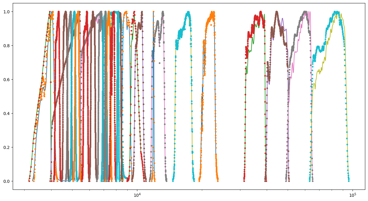
Plot the filters. We can see slight differences between those on the SVO and in the lepahre database.
[9]:
fig = plt.figure(figsize=(15, 8))
for f, fsvo in zip(filterLib, filterLibSVO):
    d = f.data()
    plt.semilogx(d[0], d[1] / d[1].max())
    dsvo = fsvo.data()
    plt.semilogx(dsvo[0], dsvo[1] / dsvo[1].max(), ".")
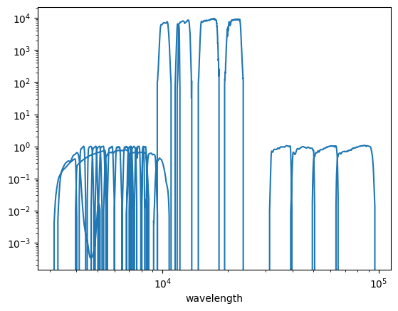
[10]:
# filter_output = os.path.join(os.environ["LEPHAREWORK"],"filt", filterLib.keymap['FILTER_FILE'] + ".dat")
# This figure shows that the filters have differing normalisation which has no impact on the fitting process.
filters = np.loadtxt(
    filter_output + ".dat", dtype={"names": ("lamb", "val", "bid"), "formats": (float, float, int)}
)
plt.loglog(filters["lamb"], filters["val"])
plt.xlabel("wavelength");
Create SED library
SED objects represent SED templates belonging to one of the three possible classes “STAR”, “QSO” (for AGN type of objects), and “GAL” for galaxies. SED templates available with LePhare can be found under the sed directory.
[11]:
sedlib = lp.Sedtolib(config_keymap=lp.all_types_to_keymap(config))
[12]:
sedlib.run(typ="STAR", star_sed="$LEPHAREDIR/sed/STAR/STAR_MOD_ALL.list")
#######################################
# It s translating SEDs to binary library #
# with the following options :
# Config file     :
# Library type     : STAR
# STAR_SED    :/home/docs/.cache/lephare/data/sed/STAR/STAR_MOD_ALL.list
# STAR_LIB    :LIB_STAR
# STAR_LIB doc:/home/docs/.cache/lephare/work/lib_bin/LIB_STAR.doc
# STAR_FSCALE :0.0000
#######################################
Number of SED in the list 254
[13]:
sedlib.run(typ="QSO", qso_sed="$LEPHAREDIR/sed/QSO/SALVATO09/AGN_MOD.list", gal_lib="LIB_QSO")
#######################################
# It s translating SEDs to binary library #
# with the following options :
# Config file     :
# Library type     : QSO
# QSO_SED    :/home/docs/.cache/lephare/data/sed/QSO/SALVATO09/AGN_MOD.list
# QSO_LIB    :LIB_QSO
# QSO_LIB doc:/home/docs/.cache/lephare/work/lib_bin/LIB_QSO.doc
# QSO_FSCALE :1.0000
#######################################
Number of SED in the list 30
[14]:
sedlib.run(typ="GAL", gal_sed="$LEPHAREDIR/sed/GAL/COSMOS_SED/COSMOS_MOD.list", gal_lib="LIB_GAL")
#######################################
# It s translating SEDs to binary library #
# with the following options :
# Config file     :
# Library type     : GAL
# GAL_SED    :/home/docs/.cache/lephare/data/sed/GAL/COSMOS_SED/COSMOS_MOD.list
# GAL_LIB    :LIB_GAL
# GAL_LIB doc:/home/docs/.cache/lephare/work/lib_bin/LIB_GAL.doc
# GAL_LIB phys:/home/docs/.cache/lephare/work/lib_bin/LIB_GAL.phys
# SEL_AGE    :none
# GAL_FSCALE :1.0000
# AGE_RANGE   0.0000 15000000000.0000
#######################################
Number of SED in the list 31
Create a magnitude library
Use the SED library to create a magnitude library
[15]:
maglib = lp.MagGal(config_keymap=lp.all_types_to_keymap(config))
[16]:
maglib.run(
    typ="STAR",
    lib_ascii="YES",
    star_lib_out="STAR_COSMOS",
    extinc_law="SB_calzetti.dat",
    mod_extinc="0,0",
)
#######################################
# It s computing the SYNTHETIC MAGNITUDES #
# For Gal/QSO libraries with these OPTIONS #
# with the following options :
# Config file     :
# Filter file     : filter_cosmos
# Magnitude type     : AB
# COSMOLOGY   :70.0000,0.3000,0.7000
# STAR_LIB_IN    :/home/docs/.cache/lephare/work/lib_bin/LIB_STAR(.doc & .bin)
# STAR_LIB_OUT   :/home/docs/.cache/lephare/work/lib_mag/STAR_COSMOS(.doc & .bin)
# LIB_ASCII   YES
# CREATION_DATE Wed Jul  1 06:05:26 2026
#############################################
[17]:
maglib.run(
    typ="QSO",
    lib_ascii="YES",
    mod_extinc="0,1000",
    eb_v="0.,0.1,0.2,0.3",
    extinc_law="SB_calzetti.dat",
    qso_lib_in="LIB_QSO",
    qso_lib_out="QSO_COSMOS",
)
#######################################
# It s computing the SYNTHETIC MAGNITUDES #
# For Gal/QSO libraries with these OPTIONS #
# with the following options :
# Config file     :
# Filter file     : filter_cosmos
# Magnitude type     : AB
# QSO_LIB_IN    :/home/docs/.cache/lephare/work/lib_bin/LIB_QSO(.doc & .bin)
# QSO_LIB_OUT   :/home/docs/.cache/lephare/work/lib_mag/QSO_COSMOS(.doc & .bin)
# Z_STEP   :0.0400 0.0000 6.0000
# COSMOLOGY   :70.0000,0.3000,0.7000
# EXTINC_LAW   :SB_calzetti.dat
# MOD_EXTINC   :0 1000
# EB_V   :0.0000 0.1000 0.2000 0.3000 # LIB_ASCII   YES
# CREATION_DATE Wed Jul  1 06:05:27 2026
#############################################
[18]:
maglib.run(
    typ="GAL",
    lib_ascii="YES",
    gal_lib_in="LIB_GAL",
    gal_lib_out="GAL_COSMOS",
    mod_extinc="18,26,26,33,26,33,26,33",
    extinc_law="SMC_prevot.dat,SB_calzetti.dat,SB_calzetti_bump1.dat,SB_calzetti_bump2.dat",
    em_lines="EMP_UV",
    em_dispersion="0.5,0.75,1.,1.5,2.",
)
#######################################
# It s computing the SYNTHETIC MAGNITUDES #
# For Gal/QSO libraries with these OPTIONS #
# with the following options :
# Config file     :
# Filter file     : filter_cosmos
# Magnitude type     : AB
# GAL_LIB_IN    :/home/docs/.cache/lephare/work/lib_bin/LIB_GAL(.doc & .bin)
# GAL_LIB_OUT   :/home/docs/.cache/lephare/work/lib_mag/GAL_COSMOS(.doc & .bin)
# Z_STEP   :0.0400 0.0000 6.0000
# COSMOLOGY   :70.0000,0.3000,0.7000
# EXTINC_LAW   :SMC_prevot.dat SB_calzetti.dat SB_calzetti_bump1.dat SB_calzetti_bump2.dat
# MOD_EXTINC   :18 26 26 33 26 33 26 33
# EB_V   :0.0000 0.1000 0.2000 0.3000
# EM_LINES   EMP_UV
# EM_DISPERSION   0.5000,0.7500,1.0000,1.5000,2.0000,
# LIB_ASCII   YES
# CREATION_DATE Wed Jul  1 06:05:44 2026
#############################################
Run the photoz
Read the parameter file and store the keywords. Example with the modification of three keywords of the parameter file. Verbose must be NO in the notebook.
[19]:
# These are the names created above with the argument gal_lib_out
config.update(
    {
        "ZPHOTLIB": "GAL_COSMOS,STAR_COSMOS,QSO_COSMOS",
        "SPEC_OUT": "save_spec",
        "AUTO_ADAPT": "YES",
        # "APPLY_SYSSHIFT": "0.049,-0.013,-0.055,-0.065,-0.042,-0.044,-0.065,-0.0156,-0.002,0.052,-0.006,0.071,0.055,0.036,0.036,0.054,0.088,0.019,-0.154,0.040,0.044,0.060,0.045,0.022,0.062,0.033,0.015,0.012,0.0,0.0]"
        "CHI2_OUT": "YES",
    }
)
Instantiate a lephare.PhotoZ object which will manage the computation of photometric redshifts for all sources. It is instantiated based on all the config parameters.
[20]:
photz = lp.PhotoZ(lp.all_types_to_keymap(config))
#######################################
# PHOTOMETRIC REDSHIFT with OPTIONS   #
# Config file            :
# CAT_IN                 : change_me_to_output_filename_required.ascii
# CAT_OUT                : zphot.out
# CAT_LINES              : 0 1000000000
# PARA_OUT               : /home/docs/.cache/lephare/data/examples/output.para
# INP_TYPE               : F
# CAT_FMT[0:MEME 1:MMEE] : 0
# CAT_MAG                : AB
# ZPHOTLIB               : GAL_COSMOS STAR_COSMOS QSO_COSMOS
# FIR_LIB                :
# FIR_LMIN               : 7.000000
# FIR_CONT               : -1.000000
# FIR_SCALE              : -1.000000
# FIR_FREESCALE          : YES
# FIR_SUBSTELLAR         : NO
# ERR_SCALE              : 0.020000 0.020000 0.020000 0.020000 0.020000 0.020000 0.020000 0.050000 0.050000 0.050000 0.050000 0.020000 0.020000 0.020000 0.020000 0.020000 0.020000 0.020000 0.020000 0.020000 0.020000 0.020000 0.020000 0.050000 0.050000 0.050000 0.050000 0.100000 0.200000 0.300000
# ERR_FACTOR             : 1.500000
# GLB_CONTEXT            : 0
# FORB_CONTEXT           : -1
# DZ_WIN                 : 1.000000
# MIN_THRES              : 0.020000
# MAG_ABS                : -24.000000 -5.000000
# MAG_ABS_AGN            : -30.000000 -10.000000
# MAG_REF                : 3
# NZ_PRIOR               : -1 -1
# Z_INTERP               : YES
# Z_METHOD               : BEST
# MABS_METHOD            : 1
# MABS_CONTEXT           : 33556478
# MABS_REF               : 11
# AUTO_ADAPT             : YES
# ADAPT_BAND             : 5
# ADAPT_LIM              : 1.500000 23.000000
# ADAPT_ZBIN             : 0.010000 6.000000
# ZFIX                   : NO
# SPEC_OUT               : save_spec
# CHI_OUT                : YES
# PDZ_OUT                : test
#######################################
Reading input librairies ...
Read lib
Number of keywords to be read in the doc: 13
Number of keywords read at the command line (excluding -c config): 0
Reading keywords from /home/docs/.cache/lephare/work/lib_mag/QSO_COSMOS.doc
Number of keywords read in the config file: 16
Keyword NUMBER_ROWS not provided
Keyword NUMBER_SED not provided
Keyword Z_FORM not provided
Reading library: /home/docs/.cache/lephare/work/lib_mag/QSO_COSMOS.bin
 Done with the library reading with 18120 SED read.
Number of keywords to be read in the doc: 13
Number of keywords read at the command line (excluding -c config): 0
Reading keywords from /home/docs/.cache/lephare/work/lib_mag/STAR_COSMOS.doc
Number of keywords read in the config file: 16
Keyword NUMBER_ROWS not provided
Keyword NUMBER_SED not provided
Keyword Z_FORM not provided
Reading library: /home/docs/.cache/lephare/work/lib_mag/STAR_COSMOS.bin
 Done with the library reading with 18374 SED read.
Number of keywords to be read in the doc: 13
Number of keywords read at the command line (excluding -c config): 0
Reading keywords from /home/docs/.cache/lephare/work/lib_mag/GAL_COSMOS.doc
Number of keywords read in the config file: 16
Keyword NUMBER_ROWS not provided
Keyword NUMBER_SED not provided
Keyword Z_FORM not provided
Reading library: /home/docs/.cache/lephare/work/lib_mag/GAL_COSMOS.bin
 Done with the library reading with 102934 SED read.
Read lib out
Read filt
# NAME                        IDENT      Lbda_mean Lbeff(Vega)       FWHM     AB-cor      VEGA   CALIB    Fac_corr
u_cfht.lowres                 1             0.3844      0.3908      0.0538    0.3150  -20.6300       0      1.0000
u_new.pb                      2             0.3690      0.3750      0.0456    0.6195  -20.8500       0      1.0000
gHSC.pb                       3             0.4851      0.4760      0.1194   -0.0860  -20.7300       0      1.0000
rHSC.pb                       4             0.6241      0.6142      0.1539    0.1466  -21.5100       0      1.0000
iHSC.pb                       5             0.7716      0.7637      0.1476    0.3942  -22.2300       0      1.0000
zHSC.pb                       6             0.8915      0.8907      0.0768    0.5169  -22.6700       0      1.0000
yHSC.pb                       7             0.9801      0.9771      0.0797    0.5534  -22.9100       0      1.0000
Y.lowres                      8             1.0220      1.0200      0.0919    0.6043  -23.0600       0      1.0000
J.lowres                      9             1.2550      1.2480      0.1712    0.9228  -23.8200       0      1.0000
H.lowres                      10            1.6500      1.6350      0.2893    1.3700  -24.8600       0      1.0000
K.lowres                      11            2.1580      2.1430      0.2926    1.8330  -25.9100       0      1.0000
IB427.lowres                  12            0.4264      0.4256      0.0207   -0.1446  -20.4100       0      1.0000
IB464.lowres                  13            0.4636      0.4633      0.0218   -0.1520  -20.5900       0      1.0000
IB484.lowres                  14            0.4851      0.4846      0.0228   -0.0241  -20.8100       0      1.0000
IB505.lowres                  15            0.5064      0.5061      0.0231   -0.0656  -20.8600       0      1.0000
IB527.lowres                  16            0.5262      0.5259      0.0242   -0.0260  -20.9900       0      1.0000
IB574.lowres                  17            0.5766      0.5762      0.0272    0.0657  -21.2800       0      1.0000
IB624.lowres                  18            0.6234      0.6230      0.0301    0.1527  -21.5300       0      1.0000
IB679.lowres                  19            0.6783      0.6779      0.0336    0.2542  -21.8200       0      1.0000
IB709.lowres                  20            0.7075      0.7071      0.0316    0.2982  -21.9500       0      1.0000
IB738.lowres                  21            0.7363      0.7358      0.0323    0.3460  -22.0900       0      1.0000
IB767.lowres                  22            0.7687      0.7681      0.0364    0.3992  -22.2400       0      1.0000
IB827.lowres                  23            0.8246      0.8241      0.0344    0.4891  -22.4800       0      1.0000
NB711.lowres                  24            0.7120      0.7119      0.0073    0.3072  -21.9800       0      1.0000
NB816.lowres                  25            0.8150      0.8149      0.0120    0.4713  -22.4300       0      1.0000
NB118.lowres                  26            1.1910      1.1910      0.0112    0.8376  -23.6200       0      1.0000
irac_ch1.lowres               27            3.5760      3.5260      0.7411    2.7950  -27.9600       1      1.0040
irac_ch2.lowres               28            4.5290      4.4610      1.0100    3.2630  -28.9400       1      1.0040
irac_ch3.lowres               29            5.7870      5.6760      1.3510    3.7540  -29.9600       1      1.0050
irac_ch4.lowres               30            8.0440      7.7030      2.8390    4.3960  -31.3000       1      1.0110
Read the input file with the following information: id, flux and associated uncertainties in all bands, a context indicating which bands to use in the fit (0 indicates all bands), and a spectrocopic redshift if it exists.
[21]:
cat = np.loadtxt(f"{lp.LEPHAREDIR}/examples/COSMOS.in")
id = cat[:, 0]
fluxes = cat[:, 1:60:2]
efluxes = cat[:, 2:61:2]
context = cat[:, 61]
zspec = cat[:, 62]
print("Check format with context and zspec :", context, zspec)
Check format with context and zspec : [0. 0. 0. ... 0. 0. 0.] [4.839 1.166 0.1649 ... 0.214 0.3053 0.3448]
Create a list of sources with a spec-z. Use for the zero-point training or any validation run.
[22]:
srclist = []
# Here, limited to the 1000 first sources.
n_obj = 100
zspec_mask = np.logical_and(zspec > 0.01, zspec < 6)
# We are running on the last n_obj objects to use a different set of objects to perform
# zero-point correction to the test objects
for i in np.where(zspec_mask)[0][-n_obj:]:
    # Each element of the list is an instance of the lephare.onesource class.
    # This encapsulates all the information for a given source.
    oneObj = lp.onesource(i, photz.gridz)
    oneObj.readsource(str(id[i]), fluxes[i, :], efluxes[i, :], int(context[i]), zspec[i], " ")
    # lephare.PhotoZ passes the configuration parameters to each source.
    photz.prep_data(oneObj)
    srclist.append(oneObj)
print("Sources with a spec-z: ", len(srclist))
Sources with a spec-z: 100
Derive the zero-points offsets. This corresponds to the median difference between apparent and observed magnitude in each filter. It is stored in the list, a0, which is later passed to the lephare.PhotoZ.run_photoz method. If AUTO_ADAPT is NO, values will be set at 0. If APPLY_SYSSHIFT is defined, that’s the values which will be used for a0.
[23]:
a0 = photz.compute_offsets(srclist)
offsets = ",".join(np.array(a0).astype(str))
offsets = "# Offsets to be added to the modeled magnitudes: " + offsets + "\n"
print(offsets)
 Done with iteration 1 and converge 0
# Offsets to be added to the modeled magnitudes: 0.10751512239554017,-0.013751160173164578,-0.04198025243697501,-0.11697590956252668,-0.09595743234742926,-0.08431394082082377,-0.10276348890739584,-0.044068619642605,-0.039664628886509234,0.017605114933900268,-0.07656523116365577,0.09369064997226317,0.05348684467240261,0.05345134781697425,0.06153858677055268,0.03245630622697604,0.06847885499805528,-0.02096930716481893,-0.1740966741636818,-0.015910269608834682,0.014805848378379949,0.03900683231785962,0.013014177355216816,-0.04133049813958323,0.040922473395568204,0.011079604090248552,-0.0745761365923947,-0.09542690832294554,0.0,0.0

 Done with iteration 2 and converge 0
 Done with iteration 3 and converge 1
Create the list of sources for which we want a photo-z.
[24]:
photozlist = []
for i in range(n_obj):
    oneObj = lp.onesource(i, photz.gridz)
    oneObj.readsource(str(id[i]), fluxes[i, :], efluxes[i, :], int(context[i]), zspec[i], " ")
    photz.prep_data(oneObj)
    photozlist.append(oneObj)
print("Number of sources to be analysed: ", len(srclist))
Number of sources to be analysed: 100
Run the photoz. We pass the values of the zero point calibration calculated above
[25]:
photz.run_photoz(photozlist, a0)
Source 95.0 // Band 14 removed to improve the chi2, with old and new chi2 502.4324 304.0052
Save the parameters that have been used
For capturing the parameters that were used in a given run it is useful to save the updated config to file. Be careful as this will not capture the overrides that were sent directly to the lephare.MagGal.run method which impact the outputs.
[26]:
# we can write the config to a file to keep a record
lp.write_para_config(lp.all_types_to_keymap(config), "./config_file.para")
# One can also save it as a yaml file if you prefer
lp.write_yaml_config(lp.all_types_to_keymap(config), "./config_file.yaml")
Create output in fits
[27]:
t = photz.build_output_tables(photozlist[:n_obj], para_out=None, filename="outputphotoz.fits")
[28]:
t[:5]
[28]:
| IDENT | Z_BEST | Z_BEST68_LOW | Z_BEST68_HIGH | Z_MED | Z_MED68_LOW | Z_MED68_HIGH | CHI_BEST | MOD_BEST | EXTLAW_BEST | EBV_BEST | Z_SEC | CHI_SEC | MOD_SEC | EBV_SEC | ZQ_BEST | CHI_QSO | MOD_QSO | MOD_STAR | CHI_STAR | MAG_OBS() | ERR_MAG_OBS() | K_COR() | MAG_ABS() | EMAG_ABS() | MABS_FILT() | SCALE_BEST | NBAND_USED | CONTEXT | ZSPEC | AGE_BEST | AGE_INF | AGE_MED | AGE_SUP | LDUST_BEST | LDUST_INF | LDUST_MED | LDUST_SUP | LUM_TIR_BEST | LUM_TIR_INF | LUM_TIR_MED | LUM_TIR_SUP | MASS_BEST | MASS_INF | MASS_MED | MASS_SUP | SFR_BEST | SFR_INF | SFR_MED | SFR_SUP | SSFR_BEST | SSFR_INF | SSFR_MED | SSFR_SUP | COL1_INF | COL1_MED | COL1_SUP | COL2_INF | COL2_MED | COL2_SUP | LUM_NUV_BEST | LUM_R_BEST | LUM_K_BEST | MAG_PRED() | STRING_INPUT | PDF_BAY_ZG() |
|---|---|---|---|---|---|---|---|---|---|---|---|---|---|---|---|---|---|---|---|---|---|---|---|---|---|---|---|---|---|---|---|---|---|---|---|---|---|---|---|---|---|---|---|---|---|---|---|---|---|---|---|---|---|---|---|---|---|---|---|---|---|---|---|---|---|
| str5 | float64 | float64 | float64 | float64 | float64 | float64 | float64 | int64 | float64 | float64 | float64 | float64 | int64 | float64 | float64 | float64 | int64 | int64 | float64 | float64[30] | float64[30] | float64[30] | float64[30] | float64[30] | float64[30] | float64 | int64 | int64 | float64 | float64 | float64 | float64 | float64 | float64 | float64 | float64 | float64 | float64 | float64 | float64 | float64 | float64 | float64 | float64 | float64 | float64 | float64 | float64 | float64 | float64 | float64 | float64 | float64 | float64 | float64 | float64 | float64 | float64 | float64 | float64 | float64 | float64 | float64[0] | str1 | float64[151] |
| 1.0 | 4.853080492769338 | 4.838848085700959 | 4.845507024036549 | 4.8410161351259005 | 4.813133637211075 | 4.86821613657054 | 37.856100061678234 | 29 | 1.0 | 0.0 | -99.9 | -99.0 | -99 | -99.0 | 4.776280077096317 | 98.02550531486065 | 29 | 204 | 135.15301956804538 | 1000.0 .. 1000.0 | 1000.0 .. 1000.0 | 966.2305682130575 .. -2.2239310754060853 | -20.483102576843944 .. -20.052866603827624 | -1.0 .. -1.0 | -1.0 .. -1.0 | 227.26284633101358 | 27 | 0 | 4.839 | -999.0 | -99.9 | -99.9 | -99.9 | -999.0 | -99.9 | -99.9 | -99.9 | -999.0 | -99.9 | -99.9 | -99.9 | -999.0 | -99.9 | -99.9 | -99.9 | -999.0 | -99.9 | -99.9 | -99.9 | -999.0 | -99.9 | -99.9 | -99.9 | -99.9 | -99.9 | -99.9 | -99.9 | -99.9 | -99.9 | 9.554660943001327 | 9.166953032216401 | 8.13254118734207 | 0.0 .. 2.4920965371441736e-42 | ||
| 2.0 | 1.189388935805745 | 1.1959067802063315 | 1.2012554603668033 | 1.1700265628526187 | 1.0693263414680285 | 1.217476509737414 | 30.093595647762406 | 18 | 1.0 | 0.1 | -99.9 | -99.0 | -99 | -99.0 | 0.966661396045455 | 24.869880911842053 | 19 | 136 | 584.518738119964 | 24.7160136546355 .. 1000.0 | 0.0964327877384378 .. 1000.0 | 0.9639373494376868 .. -0.050144543942796965 | -20.90210516937807 .. -23.422198828996468 | 0.4075378180378362 .. 3.026369808293129 | 5.0 .. 10.0 | 558.9999110522548 | 27 | 0 | 1.166 | -999.0 | -99.9 | -99.9 | -99.9 | -999.0 | -99.9 | -99.9 | -99.9 | -999.0 | -99.9 | -99.9 | -99.9 | -999.0 | -99.9 | -99.9 | -99.9 | -999.0 | -99.9 | -99.9 | -99.9 | -999.0 | -99.9 | -99.9 | -99.9 | -99.9 | -99.9 | -99.9 | -99.9 | -99.9 | -99.9 | 9.47625887700427 | 9.933577162219951 | 9.410834261790185 | 2.0568270949098572e-135 .. 0.0 | ||
| 3.0 | 0.1604570011662561 | 0.1595836914501862 | 0.16043577879533816 | 0.16 | 0.1327999997138977 | 0.1872000002861023 | 55.57302966725526 | 7 | 1.0 | 0.0 | -99.9 | -99.0 | -99 | -99.0 | 0.14921439461609912 | 121.01130963272658 | 9 | 98 | 875.937043312699 | 20.348301028072378 .. 1000.0 | 0.030183067850864845 .. 1000.0 | 0.6920535871141925 .. -0.40613677582154034 | -19.780910626629048 .. -20.358916093879184 | 0.3861506934648933 .. 2.7198853554640348 | 2.0 .. 10.0 | 150.22397059551182 | 28 | 0 | 0.1649 | -999.0 | -99.9 | -99.9 | -99.9 | -999.0 | -99.9 | -99.9 | -99.9 | -999.0 | -99.9 | -99.9 | -99.9 | -999.0 | -99.9 | -99.9 | -99.9 | -999.0 | -99.9 | -99.9 | -99.9 | -999.0 | -99.9 | -99.9 | -99.9 | -99.9 | -99.9 | -99.9 | -99.9 | -99.9 | -99.9 | 7.846166358859396 | 9.626577741958009 | 9.154315882962926 | 2.0236796113108527e-223 .. 0.0 | ||
| 4.0 | 5.654852228540542 | 5.634329965347776 | 5.678388134571853 | 5.452936926286467 | 5.291497486376177 | 5.6879022271308015 | 21.241473215194816 | 29 | 1.0 | 0.0 | -99.9 | -99.0 | -99 | -99.0 | 5.596200094324459 | 37.56644819766449 | 29 | 196 | 57.82406436425819 | 28.195532699302532 .. 1000.0 | 1.9744363436325476 .. 1000.0 | 965.841624090202 .. -2.393336073825246 | -20.96710849677425 .. -20.536872523757932 | -1.0 .. -1.0 | -1.0 .. -1.0 | 354.9202752274656 | 28 | 0 | 5.742 | -999.0 | -99.9 | -99.9 | -99.9 | -999.0 | -99.9 | -99.9 | -99.9 | -999.0 | -99.9 | -99.9 | -99.9 | -999.0 | -99.9 | -99.9 | -99.9 | -999.0 | -99.9 | -99.9 | -99.9 | -999.0 | -99.9 | -99.9 | -99.9 | -99.9 | -99.9 | -99.9 | -99.9 | -99.9 | -99.9 | 9.74826331097345 | 9.360555400188524 | 8.326143555314193 | 0.0 .. 5.790862771906528e-13 | ||
| 5.0 | 0.8667651159549735 | 0.7885401506973905 | 0.9545917146247052 | 0.9708547310919146 | 0.8059480576316304 | 1.1584984820971989 | 33.45941680386349 | 31 | 2.0 | 0.3 | -99.9 | -99.0 | -99 | -99.0 | 0.14161053989443692 | 46.23808759528594 | 4 | 136 | 99.13715198073889 | 28.43695359780653 .. 1000.0 | 2.1272798742731407 .. 1000.0 | -0.029466402861156517 .. 0.5765795031531797 | -16.202531981861835 .. -17.74346354925731 | 0.3649695029238078 .. -1.0 | 4.0 .. -1.0 | 28.44102151942098 | 28 | 0 | 5.745 | -999.0 | -99.9 | -99.9 | -99.9 | -999.0 | -99.9 | -99.9 | -99.9 | -999.0 | -99.9 | -99.9 | -99.9 | -999.0 | -99.9 | -99.9 | -99.9 | -999.0 | -99.9 | -99.9 | -99.9 | -999.0 | -99.9 | -99.9 | -99.9 | -99.9 | -99.9 | -99.9 | -99.9 | -99.9 | -99.9 | 8.750386646008867 | 8.181782088794446 | 7.085309599452671 | 0.0 .. 4.9393049955147194e-27 |
Create all ascii files with the output of the run
[29]:
import time

photz.write_outputs(photozlist[:5], int(time.time()))
[30]:
# This created the output ascii file specified in the config CAT_OUT parameter
!ls -al zphot.out
-rw-r--r-- 1 docs docs 19705 Jul 1 06:07 zphot.out
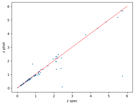
Check the results broadly follow a 1-1 relation
[31]:
plt.plot([0, 6], [0, 6], c="r", alpha=0.5)
plt.scatter(t["ZSPEC"], t["Z_BEST"], s=3)
plt.xlabel("z spec")
plt.ylabel("z phot")
[31]:
Text(0, 0.5, 'z phot')
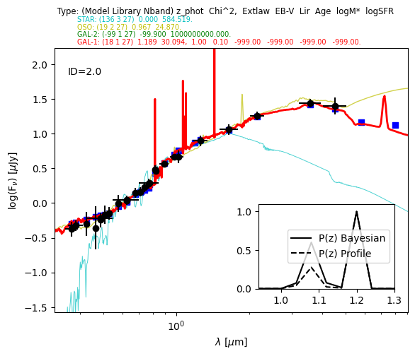
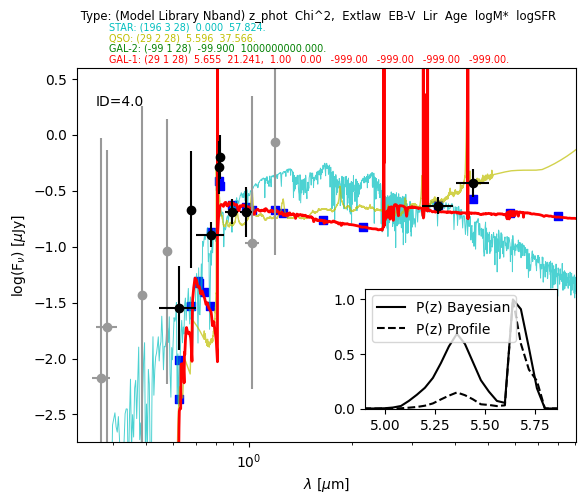
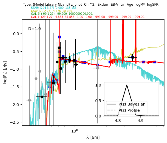
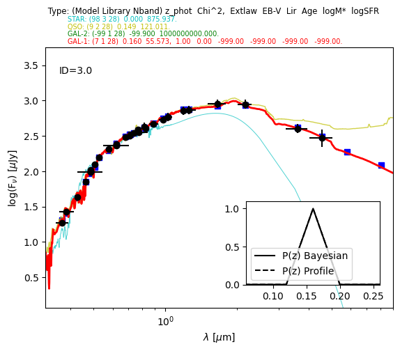
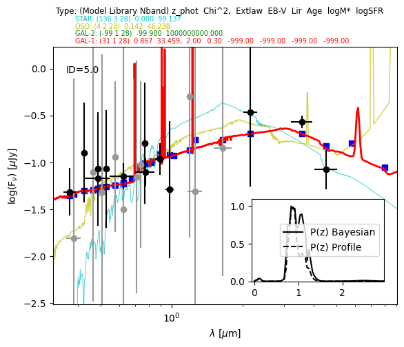
Make plots for individual sources with all the files listed in save_spec
[32]:
from os import listdir
from os.path import isfile, join

listname = [f for f in listdir("save_spec") if isfile(join("save_spec", f))]
# Lets just look at the top 10
for namefile in listname[:10]:
    lp.plotspec("save_spec/" + str(namefile))
File: save_spec/Id2.0.spec
File: save_spec/Id4.0.spec
File: save_spec/Id1.0.spec
File: save_spec/Id3.0.spec
File: save_spec/Id5.0.spec
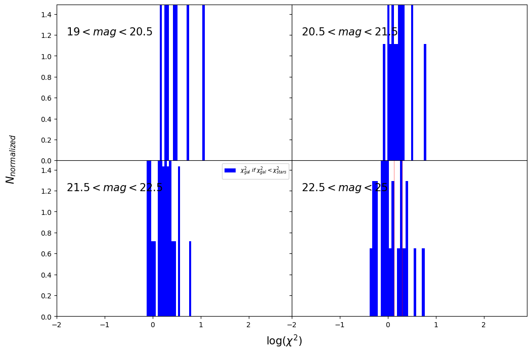
You can use some plotting utilities provided with the code. Some examples are provided below. sel_filt is the index of the filter used to select objects by observed magnitude (starting at 0). pos_filt provides the index (starting at 0) of the filters corresponding to u, g, r, z, J, and Ks bands. If you want to create all the plots and store them in a pdf file, you can use: utils.save_photoz_plots_pdf(filename=”all_photoz.pdf”)
[33]:
utils = lp.PlotUtils(
    t,
    sel_filt=4,
    pos_filt=[0, 2, 3, 5, 7, 9],
    range_z=[0, 0.5, 1, 1.5, 3],
    range_mag=[19, 20.5, 21.5, 22.5, 25],
)
[34]:
utils.dist_chi2()
<Figure size 640x480 with 0 Axes>
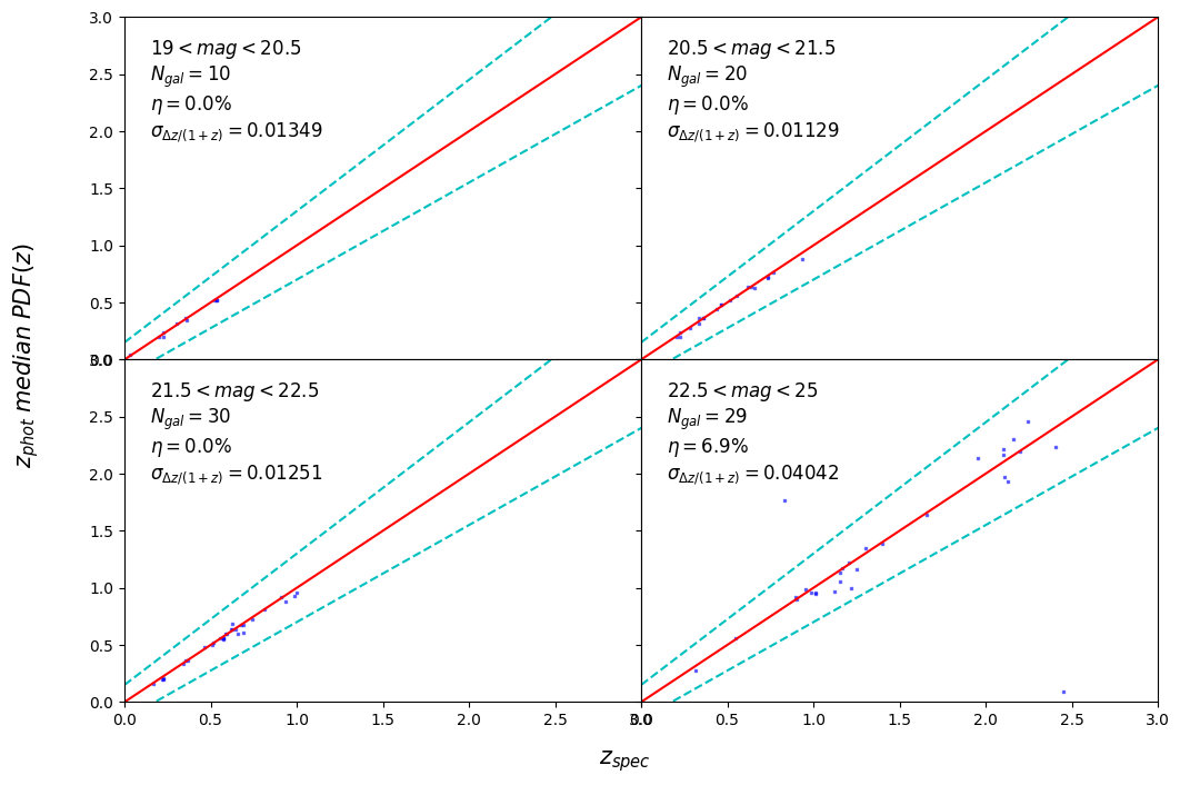
[35]:
utils.zml_zs()
<Figure size 640x480 with 0 Axes>
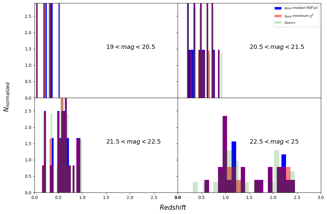
[36]:
utils.dist_z()
<Figure size 640x480 with 0 Axes>
[ ]: